Ertugliflozin (Fediuk 2021)
Source:vignettes/articles/Fediuk_2021_ertugliflozin.Rmd
Fediuk_2021_ertugliflozin.RmdModel and source
- Citation: Fediuk DJ, Zhou S, Dawra VK, Sahasrabudhe V, Sweeney K (2021). Population Pharmacokinetic Model for Ertugliflozin in Healthy Subjects and Patients With Type 2 Diabetes Mellitus. Clinical Pharmacology in Drug Development 10(7):696-706. doi:10.1002/cpdd.885.
- Description: Two-compartment population PK model for oral ertugliflozin in healthy adults and adults with type 2 diabetes mellitus, pooled across 15 phase 1-3 studies (Fediuk 2021; 2276 subjects, 13,691 concentrations). First-order absorption with a lag time and first-order elimination. Allometric body-weight scaling fixed at 0.75 on CL/F and Q/F and 1 on Vc/F and Vp/F (85 kg reference). Full-model covariate effects on CL/F (eGFR power term referenced to 90 mL/min/1.73 m^2 and capped at 120; T2DM, female sex, Black, Asian and other race), on Vc/F (age power term referenced to 65 years; female sex, Black, Asian and other race), and on absorption (fed and without-regard-to-food multipliers on ka and fractional decreases in relative bioavailability). IIV on CL/F only; log-scale additive residual error estimated separately for the phase 1 and the phase 2/3 studies.
- Article: https://doi.org/10.1002/cpdd.885 (open access; PMC8359437)
- Supplement: the Supplementary Appendix (Supporting Information file s001) holds the covariate parameterization (Equations 5-8), the study list (Table S1), the sampling schemes (Table S2) and the base-model building steps (Table S3).
Ertugliflozin is an oral sodium-glucose cotransporter 2 (SGLT2) inhibitor for type 2 diabetes mellitus (T2DM). Fediuk 2021 pooled 15 phase 1-3 studies and fitted a two-compartment model with a lag time and first-order absorption, then estimated every candidate covariate effect simultaneously (full model estimation) and reported that none was clinically relevant.
Population
The analysis data set held 13,691 ertugliflozin plasma concentrations from 2276 subjects in 9 phase 1, 2 phase 2 and 4 phase 3 studies (Table S1). Of the subjects, 2084 (91.6%) had T2DM and 192 (8.4%) were healthy. Age was 18-87 years (median 57), baseline body weight 42.6-197 kg (median 84.8), and 56.5% were male. By race 71.8% were White, 8.74% Black, 13.8% Asian and 5.62% other. MDRD eGFR had a median of 86.6 mL/min/1.73 m^2 (range 6.8-196); about 44% of subjects had normal renal function, 41% mild, 14% moderate and 1% severe renal impairment (Table 1). The phase 1 studies sampled intensively; the phase 2 and 3 studies sampled sparsely (Table S2). The phase 2 studies dosed with the morning meal, and the phase 3 studies did not record food status (dosing “without regard to food”).
The same information is available programmatically:
readModelDb("Fediuk_2021_ertugliflozin")()$population[c(
  "n_subjects", "n_studies", "age_range", "weight_range", "sex_female_pct"
)]
#> $n_subjects
#> [1] 2276
#>
#> $n_studies
#> [1] 15
#>
#> $age_range
#> [1] "18-87 years"
#>
#> $weight_range
#> [1] "42.6-197 kg"
#>
#> $sex_female_pct
#> [1] 43.5
Source trace
Every ini() value carries an in-file comment pointing to
its source in
inst/modeldb/specificDrugs/Fediuk_2021_ertugliflozin.R. The
table collects them. All estimates are the final-model column of Table
2.
| Equation / parameter | Value | Source location |
|---|---|---|
lcl (CL/F) |
log(12.0) L/h | Table 2 |
lvc (Vc/F) |
log(6.54) L | Table 2 |
lvp (Vp/F) |
log(107) L | Table 2 |
lq (Q/F) |
log(7.77) L/h | Table 2 |
lka (ka, fasted) |
log(0.329) 1/h | Table 2 |
ltlag (lag time) |
log(0.228) h | Table 2 |
lfdepot (F1, fasted) |
fixed(log(1)) | Table 2 (1.00 FIX) |
e_wt_cl_q |
fixed(0.75) | Table 2 (0.750 FIX on CL/F and Q/F) |
e_wt_vc_vp |
fixed(1) | Table 2 (1.00 FIX on Vc/F and Vp/F) |
e_crcl_cl |
0.455 | Table 2, CL/F ‘Effect of eGFR’ |
e_dis_diab_cl |
0.904 | Table 2, CL/F ‘Effect of T2DM patient status’ |
e_sexf_cl |
0.962 | Table 2, CL/F ‘Effect of female sex’ |
e_race_black_cl / e_race_asian_cl /
e_race_other_cl
|
0.985 / 1.08 / 0.992 | Table 2, CL/F race rows |
e_age_vc |
-0.243 | Table 2, Vc/F ‘Effect of age’ |
e_sexf_vc |
1.36 | Table 2, Vc/F ‘Effect of female sex’ |
e_race_black_vc / e_race_asian_vc /
e_race_other_vc
|
0.917 / 2.12 / 1.15 | Table 2, Vc/F race rows |
e_fed_ka / e_fed_missing_ka
|
0.726 / 0.663 | Table 2, ka food rows |
e_fed_fdepot / e_fed_missing_fdepot
|
0.0683 / 0.0809 | Table 2, F1 food rows |
etalcl |
0.102 (variance) | Table 2, omega^2 (CL/F); 32% CV in Results |
expSdPh1 / expSdPh23
|
0.387 / 0.836 | Table 2 residual rows; 38.7% and 83.6% in Results |
Continuous covariates (cov/ref)^theta, refs 85 kg, 65
y, 90 mL/min/1.73 m^2 |
n/a | Supplementary Appendix Equation 5 |
Categorical covariates theta^cov
|
n/a | Supplementary Appendix Equation 6 |
F1 = 1 - FED*theta - FED_MISSING*theta |
n/a | Supplementary Appendix Equations 7-8 |
| CL/F, Vc/F, Vp/F, Q/F, ka, F1 covariate model | n/a | Supplementary Appendix Equation 8 |
| eGFR capped at 120 mL/min/1.73 m^2 | n/a | Methods, Covariate Evaluation |
Cc ~ lnorm() (additive on log concentration) |
n/a | Supplementary Appendix Equation 4 |
| 2-compartment ODEs, lag time, first-order absorption | n/a | Methods, PopPK Model |
Typical-value covariate checks
The Results section translates the covariate effects into typical-value statements relative to a reference subject: a 65-year-old healthy White man weighing 85 kg with an eGFR of 90 mL/min/1.73 m^2, dosed fasted. Those statements depend on no random effect, so the packaged model must reproduce them to within the paper’s own rounding.
mod <- readModelDb("Fediuk_2021_ertugliflozin")
# Random effects set to zero; later chunks supply the CL/F random effect as
# a data column where between-subject variability is wanted.
mod_typical <- rxode2::zeroRe(mod)
#> ℹ parameter labels from comments will be replaced by 'label()'
#> Warning: No sigma parameters in the model

ref_subject <- tibble(
  WT = 85, AGE = 65, CRCL = 90, DIS_DIAB = 0, SEXF = 0,
  RACE_BLACK = 0, RACE_ASIAN = 0, RACE_OTHER = 0,
  FED = 0, FED_MISSING = 0, STUDY_PHASE2 = 0, STUDY_PHASE3 = 0
)

scenarios <- bind_rows(
  ref_subject |> mutate(scenario = "Reference"),
  ref_subject |> mutate(scenario = "WT 59.5 kg", WT = 59.5),
  ref_subject |> mutate(scenario = "WT 123 kg", WT = 123),
  ref_subject |> mutate(scenario = "eGFR 60", CRCL = 60),
  ref_subject |> mutate(scenario = "eGFR 45", CRCL = 45),
  ref_subject |> mutate(scenario = "eGFR 150 (capped at 120)", CRCL = 150),
  ref_subject |> mutate(scenario = "eGFR 120", CRCL = 120),
  ref_subject |> mutate(scenario = "T2DM", DIS_DIAB = 1),
  ref_subject |> mutate(scenario = "Female", SEXF = 1),
  ref_subject |> mutate(scenario = "Asian", RACE_ASIAN = 1),
  ref_subject |> mutate(scenario = "Fed", FED = 1),
  ref_subject |> mutate(scenario = "Without regard to food", FED_MISSING = 1)
) |>
  mutate(id = row_number())

# One 15 mg dose per scenario plus a dense grid on the central compartment;
# the algebraic outputs cl, vc, vp, q, ka and fdepot come back per row.
typ_events <- scenarios |>
  tidyr::crossing(time = c(0, seq(0.05, 96, by = 0.05))) |>
  mutate(
    evid = ifelse(time == 0, 1L, 0L),
    amt = ifelse(evid == 1L, 15, 0),
    cmt = ifelse(evid == 1L, "depot", "central")
  ) |>
  bind_rows(scenarios |> mutate(time = 0, evid = 0L, amt = 0, cmt = "central")) |>
  arrange(id, time, desc(evid))

typ <- rxode2::rxSolve(
  mod_typical, typ_events, returnType = "data.frame",
  keep = "scenario"
)
#> ℹ omega/sigma items treated as zero: 'etalcl'
#> Warning: multi-subject simulation without without 'omega'

typ_par <- typ |>
  group_by(scenario) |>
  summarise(
    cl = first(cl), vc = first(vc), vp = first(vp), q = first(q),
    ka = first(ka), fdepot = first(fdepot),
    cmax = max(Cc), tmax = time[which.max(Cc)],
    .groups = "drop"
  ) |>
  mutate(auc_tau_ss = 15 * fdepot / cl * 1000) # ng*h/mL, = AUCinf single dose

ref_row <- typ_par |> filter(scenario == "Reference")
typ_par <- typ_par |>
  mutate(
    cl_ratio = cl / ref_row$cl,
    auc_ratio = auc_tau_ss / ref_row$auc_tau_ss,
    vc_ratio = vc / ref_row$vc,
    ka_ratio = ka / ref_row$ka
  )

typ_par |>
  select(scenario, cl, vc, vp, q, ka, fdepot, cl_ratio, auc_ratio, vc_ratio) |>
knitr::kable(digits = 3, caption = "Typical-value parameters by scenario.")| scenario | cl | vc | vp | q | ka | fdepot | cl_ratio | auc_ratio | vc_ratio |
|---|---|---|---|---|---|---|---|---|---|
| Asian | 12.960 | 13.865 | 107.000 | 7.770 | 0.329 | 1.000 | 1.080 | 0.926 | 2.120 |
| Fed | 12.000 | 6.540 | 107.000 | 7.770 | 0.239 | 0.932 | 1.000 | 0.932 | 1.000 |
| Female | 11.544 | 8.894 | 107.000 | 7.770 | 0.329 | 1.000 | 0.962 | 1.040 | 1.360 |
| Reference | 12.000 | 6.540 | 107.000 | 7.770 | 0.329 | 1.000 | 1.000 | 1.000 | 1.000 |
| T2DM | 10.848 | 6.540 | 107.000 | 7.770 | 0.329 | 1.000 | 0.904 | 1.106 | 1.000 |
| WT 123 kg | 15.832 | 9.464 | 154.835 | 10.251 | 0.329 | 1.000 | 1.319 | 0.758 | 1.447 |
| WT 59.5 kg | 9.183 | 4.578 | 74.900 | 5.946 | 0.329 | 1.000 | 0.765 | 1.307 | 0.700 |
| Without regard to food | 12.000 | 6.540 | 107.000 | 7.770 | 0.218 | 0.919 | 1.000 | 0.919 | 1.000 |
| eGFR 120 | 13.678 | 6.540 | 107.000 | 7.770 | 0.329 | 1.000 | 1.140 | 0.877 | 1.000 |
| eGFR 150 (capped at 120) | 13.678 | 6.540 | 107.000 | 7.770 | 0.329 | 1.000 | 1.140 | 0.877 | 1.000 |
| eGFR 45 | 8.754 | 6.540 | 107.000 | 7.770 | 0.329 | 1.000 | 0.730 | 1.371 | 1.000 |
| eGFR 60 | 9.978 | 6.540 | 107.000 | 7.770 | 0.329 | 1.000 | 0.832 | 1.203 | 1.000 |
The paper’s weight statements (Results, Parameter Estimate Results) cover the 5th and 95th percentiles of observed body weight, 59.5 and 123 kg.
published_wt <- tribble(
  ~scenario,    ~parameter, ~published,
  "WT 59.5 kg", "cl",       9.18,
  "WT 123 kg",  "cl",       15.8,
  "WT 59.5 kg", "vc",       4.58,
  "WT 123 kg",  "vc",       9.46,
  "WT 59.5 kg", "vp",       75,
  "WT 123 kg",  "vp",       155,
  "WT 59.5 kg", "q",        5.95,
  "WT 123 kg",  "q",        10.3
)
wt_check <- published_wt |>
  left_join(
    typ_par |>
      select(scenario, cl, vc, vp, q) |>
      pivot_longer(-scenario, names_to = "parameter", values_to = "model"),
    by = c("scenario", "parameter")
  ) |>
  mutate(pct_diff = 100 * (model / published - 1))

wt_check |>
  rename(
    "Scenario" = scenario, "Parameter" = parameter,
    "Published" = published, "Model" = model, "% difference" = pct_diff
  ) |>
knitr::kable(digits = 2, caption = "Body-weight extremes: model vs Results text.")| Scenario | Parameter | Published | Model | % difference |
|---|---|---|---|---|
| WT 59.5 kg | cl | 9.18 | 9.18 | 0.04 |
| WT 123 kg | cl | 15.80 | 15.83 | 0.20 |
| WT 59.5 kg | vc | 4.58 | 4.58 | -0.04 |
| WT 123 kg | vc | 9.46 | 9.46 | 0.04 |
| WT 59.5 kg | vp | 75.00 | 74.90 | -0.13 |
| WT 123 kg | vp | 155.00 | 154.84 | -0.11 |
| WT 59.5 kg | q | 5.95 | 5.95 | -0.06 |
| WT 123 kg | q | 10.30 | 10.25 | -0.47 |
# Deterministic: the only error is the paper's 3-significant-figure rounding
# (largest 0.5%, Q at 123 kg: 10.25 vs 10.3).
stopifnot(all(abs(wt_check$pct_diff) < 1))
The AUC and volume ratios are the paper’s Figure 3 statements: AUCtau is 20% and 37% higher at an eGFR of 60 and 45 mL/min/1.73 m^2; 11% higher in T2DM, 4% higher in women and 7% lower in Asians; Vc/F is 36% higher in women and 112% higher in Asians. The food statements are Table 2 read as percent decreases: ka falls about 27% (fed) and 34% (without regard to food), and F1 about 7% and 8%.
published_ratio <- tribble(
  ~scenario,                ~quantity,   ~published,
  "eGFR 60",                "auc_ratio", 1.20,
  "eGFR 45",                "auc_ratio", 1.37,
  "T2DM",                   "auc_ratio", 1.11,
  "Female",                 "auc_ratio", 1.04,
  "Asian",                  "auc_ratio", 0.93,
  "Female",                 "vc_ratio",  1.36,
  "Asian",                  "vc_ratio",  2.12,
  "Fed",                    "ka_ratio",  0.73,
  "Without regard to food", "ka_ratio",  0.66,
  "Fed",                    "fdepot",    0.93,
  "Without regard to food", "fdepot",    0.92
)
ratio_check <- published_ratio |>
  left_join(
    typ_par |>
      select(scenario, auc_ratio, vc_ratio, ka_ratio, fdepot) |>
      pivot_longer(-scenario, names_to = "quantity", values_to = "model"),
    by = c("scenario", "quantity")
  ) |>
  mutate(abs_diff = model - published)

ratio_check |>
  rename(
    "Scenario" = scenario, "Quantity" = quantity,
    "Published" = published, "Model" = model, "Difference" = abs_diff
  ) |>
knitr::kable(digits = 3, caption = "Covariate ratios: model vs Results text and Figure 3.")| Scenario | Quantity | Published | Model | Difference |
|---|---|---|---|---|
| eGFR 60 | auc_ratio | 1.20 | 1.203 | 0.003 |
| eGFR 45 | auc_ratio | 1.37 | 1.371 | 0.001 |
| T2DM | auc_ratio | 1.11 | 1.106 | -0.004 |
| Female | auc_ratio | 1.04 | 1.040 | 0.000 |
| Asian | auc_ratio | 0.93 | 0.926 | -0.004 |
| Female | vc_ratio | 1.36 | 1.360 | 0.000 |
| Asian | vc_ratio | 2.12 | 2.120 | 0.000 |
| Fed | ka_ratio | 0.73 | 0.726 | -0.004 |
| Without regard to food | ka_ratio | 0.66 | 0.663 | 0.003 |
| Fed | fdepot | 0.93 | 0.932 | 0.002 |
| Without regard to food | fdepot | 0.92 | 0.919 | -0.001 |
# Deterministic: published values are rounded to two decimals, so every
# difference must sit inside half a unit in the second place plus a margin.
stopifnot(all(abs(ratio_check$abs_diff) < 0.01))

# The eGFR cap: any value above 120 gives the eGFR-120 clearance.
stopifnot(
  isTRUE(all.equal(
    typ_par$cl[typ_par$scenario == "eGFR 150 (capped at 120)"],
    typ_par$cl[typ_par$scenario == "eGFR 120"]
  ))
)
The Results also report a mean elimination half-life of 15.3 hours for healthy subjects and 16.6 hours for patients with T2DM and normal renal function. The terminal half-life of the typical reference subject, and of the same subject with T2DM, follows in closed form from the two-compartment micro-constants.
terminal_half_life <- function(cl, vc, vp, q) {
  k10 <- cl / vc
  k12 <- q / vc
  k21 <- q / vp
  s <- k10 + k12 + k21
  beta <- (s - sqrt(s^2 - 4 * k10 * k21)) / 2
  log(2) / beta
}
hl <- typ_par |>
  filter(scenario %in% c("Reference", "T2DM")) |>
  mutate(
    half_life = terminal_half_life(cl, vc, vp, q),
    published = c(Reference = 15.3, T2DM = 16.6)[scenario],
    pct_diff = 100 * (half_life / published - 1)
  ) |>
  select(scenario, half_life, published, pct_diff)
hl |>
  rename(
    "Scenario" = scenario, "Model t1/2 (h)" = half_life,
    "Published mean t1/2 (h)" = published, "% difference" = pct_diff
  ) |>
knitr::kable(digits = 2, caption = "Terminal half-life: typical subject vs published mean.")| Scenario | Model t1/2 (h) | Published mean t1/2 (h) | % difference |
|---|---|---|---|
| Reference | 15.88 | 15.3 | 3.77 |
| T2DM | 16.56 | 16.6 | -0.25 |
The typical-subject half-life is not the same statistic as the paper’s mean of individual half-lives (a mean over subjects of varying eGFR, weight, sex and race), so the agreement is expected to be close but not exact; the check below allows 10%.
Virtual cohort
Original observed data are not publicly available. The virtual population approximates Table 1: body weight, age and eGFR drawn from truncated normal distributions with the published means and SDs, and sex, race and T2DM status drawn at the published proportions.
set.seed(20210701)
stopifnot(isTRUE(all.equal(unname(rxode2::rxode(mod)$omega[1, 1]), 0.102)))
#> ℹ parameter labels from comments will be replaced by 'label()'

rtnorm <- function(n, mean, sd, lo, hi) {
  x <- rnorm(n, mean, sd)
  bad <- x < lo | x > hi
  while (any(bad)) {
    x[bad] <- rnorm(sum(bad), mean, sd)
    bad <- x < lo | x > hi
  }
  x
}

make_cohort <- function(n, dose, id_offset = 0L) {
  race <- sample(
    c("White", "Black", "Asian", "Other"), n,
    replace = TRUE, prob = c(71.8, 8.74, 13.8, 5.62)
  )
  subj <- tibble(
    id = id_offset + seq_len(n),
    treatment = paste(dose, "mg QD"),
    WT = rtnorm(n, 86.9, 19.7, 42.6, 197),
    AGE = rtnorm(n, 55.7, 11.6, 18, 87),
    CRCL = rtnorm(n, 85.9, 24.3, 6.8, 196),
    SEXF = rbinom(n, 1, 0.435),
    RACE_BLACK = as.integer(race == "Black"),
    RACE_ASIAN = as.integer(race == "Asian"),
    RACE_OTHER = as.integer(race == "Other"),
    DIS_DIAB = 1L,
    FED = 0L, FED_MISSING = 0L,
    STUDY_PHASE2 = 0L, STUDY_PHASE3 = 0L,
    # CL/F random effect drawn in R (Table 2 omega^2 = 0.102) and supplied
    # as a data column to the zeroRe() model, so the cohort does not depend
    # on rxode2's per-thread random-number streams.
    etalcl = rnorm(n, 0, sqrt(0.102))
  )
  # Seven once-daily doses (steady state is reached well within a week for
  # a ~16 h half-life), then an intensively sampled day-7 interval and a
  # 72 h washout tail, as in the phase 1 multiple-dose studies (Table S2).
  doses <- subj |>
    tidyr::crossing(time = seq(0, 144, by = 24)) |>
    mutate(evid = 1L, amt = dose, cmt = "depot")
  obs_times <- c(0, 0.5, 1, 1.5, 2, 3, 4, 6, 8, 12, 24, seq(144, 216, by = 0.5))
  obs <- subj |>
    tidyr::crossing(time = sort(unique(obs_times))) |>
    mutate(evid = 0L, amt = 0, cmt = "central")
  bind_rows(doses, obs) |> arrange(id, time, desc(evid))
}

events <- bind_rows(
  make_cohort(200, dose = 5, id_offset = 0L),
  make_cohort(200, dose = 15, id_offset = 200L)
)
stopifnot(!anyDuplicated(unique(events[, c("id", "time", "evid")])))
Simulation
sim <- rxode2::rxSolve(
  mod_typical, events = events, keep = c("treatment"),
  returnType = "data.frame"
)
#> ℹ omega/sigma items treated as zero: 'etalcl'
#> Warning: multi-subject simulation without without 'omega'
Cc is the individual prediction (IPRED)
given each subject’s covariates and drawn CL/F random effect; residual
error is not added.
Replicate published figures
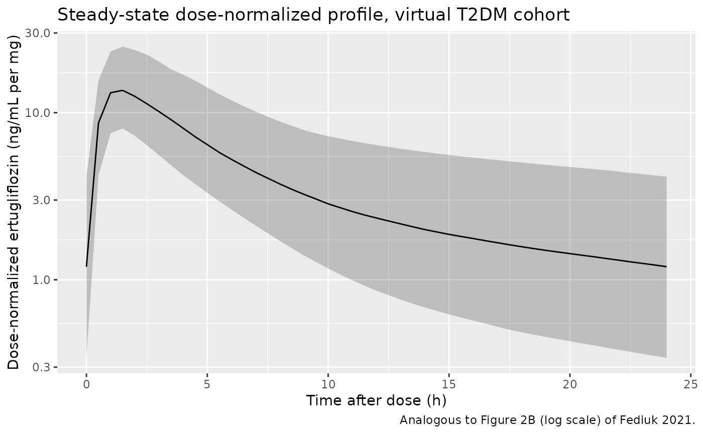
Figure 2 of Fediuk 2021 is a visual predictive check of dose-normalized concentration against time after dose, pooled across the 15 studies. The pooled observed data are not reproducible, so the analogous panel below shows the dose-normalized day-7 steady-state profile of the virtual T2DM cohort, with the median and 95% prediction interval.
sim |>
  filter(time >= 144, time <= 168) |>
  mutate(
    tad = time - 144,
    dn = Cc / ifelse(treatment == "5 mg QD", 5, 15)
  ) |>
  group_by(tad) |>
  summarise(
    Q025 = quantile(dn, 0.025),
    Q50 = median(dn),
    Q975 = quantile(dn, 0.975),
    .groups = "drop"
  ) |>
  ggplot(aes(tad, Q50)) +
  geom_ribbon(aes(ymin = Q025, ymax = Q975), alpha = 0.25) +
  geom_line() +
  scale_y_log10() +
  labs(
    x = "Time after dose (h)",
    y = "Dose-normalized ertugliflozin (ng/mL per mg)",
    title = "Steady-state dose-normalized profile, virtual T2DM cohort",
    caption = "Analogous to Figure 2B (log scale) of Fediuk 2021."
  )
PKNCA validation
Steady state, 5 and 15 mg once daily
ss_conc <- sim |>
  filter(!is.na(Cc), time >= 144) |>
  mutate(Cc = pmax(Cc, 0)) |>
  select(id, time, Cc, treatment)

ss_dose <- events |>
  filter(evid == 1) |>
  select(id, time, amt, treatment)

conc_obj <- PKNCA::PKNCAconc(ss_conc, Cc ~ time | treatment + id)
dose_obj <- PKNCA::PKNCAdose(ss_dose, amt ~ time | treatment + id)
# Day-7 dosing interval for exposure; the 72 h washout after the last dose
# for the terminal half-life.
intervals_ss <- data.frame(
  start = c(144, 144), end = c(168, 216),
  cmax = c(TRUE, FALSE), tmax = c(TRUE, FALSE),
  auclast = c(TRUE, FALSE), cav = c(TRUE, FALSE),
  half.life = c(FALSE, TRUE)
)
nca_ss <- PKNCA::pk.nca(PKNCA::PKNCAdata(
  conc_obj, dose_obj,
  intervals = intervals_ss
))
# Select each metric from its own interval: requesting half.life on the
# washout interval also emits companion rows (e.g. tmax) for that interval,
# which a group_by(PPTESTCD) summary would otherwise pool silently.
nca_ss_ind <- as.data.frame(nca_ss$result) |>
  filter(
    (end == 168 & PPTESTCD %in% c("cmax", "tmax", "auclast", "cav")) |
      (end == 216 & PPTESTCD == "half.life")
  )
stopifnot(
  !anyDuplicated(nca_ss_ind[, c("id", "PPTESTCD")]),
  nrow(nca_ss_ind) == 5 * length(unique(ss_conc$id))
)
nca_ss_summary <- nca_ss_ind |>
  group_by(treatment, PPTESTCD) |>
  summarise(median = median(PPORRES, na.rm = TRUE), .groups = "drop") |>
  pivot_wider(names_from = PPTESTCD, values_from = median)

nca_ss_summary |>
  rename(
    "Regimen" = treatment,
    "Cmax (ng/mL)" = cmax,
    "Tmax (h)" = tmax,
    "AUCtau (ng*h/mL)" = auclast,
    "Cav (ng/mL)" = cav,
    "t1/2 (h)" = half.life
  ) |>
knitr::kable(digits = 1, caption = "Median steady-state NCA of the virtual T2DM cohort.")| Regimen | AUCtau (ng*h/mL) | Cav (ng/mL) | Cmax (ng/mL) | t1/2 (h) | Tmax (h) |
|---|---|---|---|---|---|
| 15 mg QD | 1421.8 | 59.2 | 201.8 | 16.8 | 1.5 |
| 5 mg QD | 478.8 | 20.0 | 69.6 | 16.8 | 1.5 |
The model is linear, so the exposure must be dose-proportional, and the median PKNCA half-life of this T2DM cohort (mixed renal function) should sit near the published 16.6 h for T2DM patients with normal renal function.
auc_by_dose <- setNames(nca_ss_summary$auclast, nca_ss_summary$treatment)
# Two independent 200-subject cohorts: the dose-normalized median AUC ratio
# is 1 in expectation; the between-cohort spread of the median is a few
# percent at 32% CV on CL/F.
stopifnot(
  abs(auc_by_dose[["15 mg QD"]] / (3 * auc_by_dose[["5 mg QD"]]) - 1) < 0.1,
  abs(median(nca_ss_summary$half.life) / 16.6 - 1) < 0.15
)
Food effect, single 15 mg dose
The Discussion compares the model’s food effects with a phase 1 food-effect study (study I-8, 15 mg single dose in healthy subjects), in which the fed state lowered Cmax by 29%, delayed median Tmax by 1 hour and lowered AUCinf by about 8%. The same subjects are simulated here under both prandial states by passing each subject’s CL/F random effect as a data column, so the fed-to-fasted ratios are paired within subject.
n_food <- 200
food_subj <- tibble(
  id = seq_len(n_food),
  WT = rtnorm(n_food, 75, 12, 50, 110),
  AGE = rtnorm(n_food, 35, 10, 18, 55),
  CRCL = rtnorm(n_food, 105, 15, 80, 196),
  SEXF = rbinom(n_food, 1, 0.3),
  RACE_BLACK = 0L, RACE_ASIAN = 0L, RACE_OTHER = 0L,
  DIS_DIAB = 0L, FED_MISSING = 0L, STUDY_PHASE2 = 0L, STUDY_PHASE3 = 0L,
  etalcl = rnorm(n_food, 0, sqrt(0.102))
)
food_events <- bind_rows(
  food_subj |> mutate(treatment = "Fasted", FED = 0L),
  food_subj |> mutate(treatment = "Fed", FED = 1L, id = id + n_food)
) |>
  tidyr::crossing(time = c(seq(0, 6, by = 0.25), 8, 10, 12, 16, 24, 36, 48, 72, 96)) |>
  mutate(evid = 0L, amt = 0, cmt = "central")
food_events <- bind_rows(
  food_events,
  food_events |>
    distinct(id, .keep_all = TRUE) |>
    mutate(time = 0, evid = 1L, amt = 15, cmt = "depot")
) |>
  arrange(id, time, desc(evid))

food_sim <- rxode2::rxSolve(
  mod_typical, food_events, keep = "treatment",
  returnType = "data.frame"
)
#> ℹ omega/sigma items treated as zero: 'etalcl'
#> Warning: multi-subject simulation without without 'omega'

food_conc <- food_sim |>
  filter(!is.na(Cc)) |>
  mutate(Cc = pmax(Cc, 0)) |>
  select(id, time, Cc, treatment)
food_dose <- food_events |>
  filter(evid == 1) |>
  select(id, time, amt, treatment)

nca_food <- PKNCA::pk.nca(PKNCA::PKNCAdata(
  PKNCA::PKNCAconc(food_conc, Cc ~ time | treatment + id),
  PKNCA::PKNCAdose(food_dose, amt ~ time | treatment + id),
  intervals = data.frame(start = 0, end = Inf, cmax = TRUE, tmax = TRUE, aucinf.obs = TRUE)
))

food_ind <- as.data.frame(nca_food$result) |>
  filter(PPTESTCD %in% c("cmax", "tmax", "aucinf.obs")) |>
  mutate(subject = ifelse(id > n_food, id - n_food, id)) |>
  select(subject, treatment, PPTESTCD, PPORRES) |>
  pivot_wider(names_from = treatment, values_from = PPORRES)

food_summary <- food_ind |>
  group_by(PPTESTCD) |>
  summarise(
    model = ifelse(
      first(PPTESTCD) == "tmax",
      median(Fed) - median(Fasted),
      exp(mean(log(Fed / Fasted)))
    ),
    .groups = "drop"
  ) |>
  mutate(
    published = c(aucinf.obs = 0.92, cmax = 0.71, tmax = 1)[PPTESTCD],
    statistic = ifelse(
      PPTESTCD == "tmax", "median Tmax difference (h)", "geometric mean ratio fed/fasted"
    )
  ) |>
  select(PPTESTCD, statistic, model, published)

food_summary |>
  rename(
    "NCA parameter" = PPTESTCD, "Statistic" = statistic,
    "Model" = model, "Published (study I-8)" = published
  ) |>
knitr::kable(digits = 2, caption = "Food effect, 15 mg single dose: model vs Discussion.")| NCA parameter | Statistic | Model | Published (study I-8) |
|---|---|---|---|
| aucinf.obs | geometric mean ratio fed/fasted | 0.93 | 0.92 |
| cmax | geometric mean ratio fed/fasted | 0.72 | 0.71 |
| tmax | median Tmax difference (h) | 0.00 | 1.00 |
fe <- setNames(food_summary$model, food_summary$PPTESTCD)
stopifnot(
  # AUC ratio is exactly 1 - 0.0683 per subject (linear model, paired CL/F);
  # the published ~8% decrease is a separate NCA study, rounded.
  abs(fe[["aucinf.obs"]] - 0.9317) < 0.005,
  # Cmax: the typical reference subject gives 0.715 (0.05 h grid, above); the
  # paired cohort ratio depends only weakly on CL/F and weight. The Discussion
  # reports a 29% decrease (ratio 0.71).
  abs(fe[["cmax"]] - 0.71) < 0.05
)
The simulated AUCinf ratio is 0.93, in line with the published 8% decrease, and the Cmax ratio of 0.72 reproduces the 29% Cmax decrease of the dedicated food-effect study. The model’s median Tmax delay is 0 h on this 0.25 h grid (0.25 h for the typical subject on the 0.05 h grid above) against the observed median delay of 1 hour. The pooled model carries a single lag time for all prandial states and slows only ka with food, so it does not reproduce the full Tmax shift of a standardized food-effect crossover; Tmax is shown as a descriptive comparison and is not gated.
Assumptions and deviations
-
Residual error is on the SD scale. Table 2 labels
the two residual rows only ‘residual error’ (0.387 and 0.836), while it
labels the IIV row explicitly as a variance (omega^2 0.102). The Results
report the residual errors as 38.7% and 83.6% and the IIV as 32%,
i.e. the authors took the square root of the variance for the IIV but
not for the residual rows. The residual values are therefore read as
log-scale SDs and used directly in
lnorm(). -
The phase 2 and phase 3 studies share one residual
SD. The model selects it when either
STUDY_PHASE2orSTUDY_PHASE3is 1; set both to 0 (phase 1 residual) for a richly sampled profile. -
“Without regard to food” is a missing-food-status
stratum. The phase 3 studies did not document food intake, so
the corresponding indicator is encoded as
FED_MISSING, not as a meal type. Use it only to reproduce the phase 3 setting; simulate a defined fasted or fed state withFED_MISSING = 0. -
eGFR cap. The authors set eGFR values above 120
mL/min/1.73 m^2 to 120 in the data set;
model()applies the same cap, so users can supply uncapped eGFR. - Virtual cohort. Body weight, age and eGFR were drawn from truncated normal distributions with the Table 1 means, SDs and ranges, independently of each other; the paper reports a correlation of -0.531 between age and eGFR that the cohort does not reproduce. Every virtual subject in the steady-state cohort has T2DM. The food-effect cohort’s demographics (young healthy adults) are assumptions, since study I-8 demographics are not reported in the paper.
- Base model not packaged. Table 2 also reports the final base model (no covariates beyond weight and food). Only the final model is packaged.
- No erratum was found for this article (Europe PMC search, 2026-09-28).