COVID-19 vaccine immune correlates of protection (Kandala 2022) • nlmixr2lib

Model and source

Citation: Kandala B, Plock N, Chawla A, Largajolli A, Robey S, Watson K, et al. Accelerating model-informed decisions for COVID-19 vaccine candidates using a model-based meta-analysis approach. EBioMedicine. 2022;84:104264. doi:10.1016/j.ebiom.2022.104264.
Article: https://doi.org/10.1016/j.ebiom.2022.104264

This paper is a model-based meta-analysis (MBMA), not a population PK analysis. It builds a translational framework linking a vaccine’s serum neutralizing (SN) titre to protection, first in rhesus macaques (RM) and then in humans. The unit of observation is a published study-arm summary, and the models are weighted (non-)linear mixed-effects / generalized-least-squares meta-regressions with no time course, no dosing and no concentrations. There is therefore no PKNCA section in this vignette; the validation below replaces it with structural (closed-form) checks, exact replication of the paper’s own published predictions (the 50% protective titres, the Table 4 external validation, and the Table 5 delta-variant predictions), and figure reproductions.

The paper develops four models, extracted as four files:

Model file	Paper’s role	Driver	Output
`Kandala_2022_covid19Vaccine_rm_mbma`	RM MBMA (Table 2)	log2 SN titre	`log10_viral_load`
`Kandala_2022_covid19Vaccine_calibrated_mbma`	Calibrated RM MBMA (Figure 3)	SN/HCS ratio	`ve` (%)
`Kandala_2022_covid19Vaccine_joint_mbma`	Joint RM+clinical MBMA (Figure 4)	log2 SN (RM) / SN/HCS (human)	`ve` (%)
`Kandala_2022_covid19Vaccine_clinical_mbma`	Clinical MBMA (Figure 5)	SN/HCS ratio	`ve` (%)

mod_rm    <- readModelDb("Kandala_2022_covid19Vaccine_rm_mbma")
mod_cal   <- readModelDb("Kandala_2022_covid19Vaccine_calibrated_mbma")
mod_joint <- readModelDb("Kandala_2022_covid19Vaccine_joint_mbma")
mod_clin  <- readModelDb("Kandala_2022_covid19Vaccine_clinical_mbma")

# Typical-value copy of the one model that carries a random effect (the RM
# MBMA's study-level eta on VLmax). The three efficacy models have no random
# effects, so they are already deterministic.
tv_rm <- rxode2::zeroRe(mod_rm)
#> ℹ parameter labels from comments will be replaced by 'label()'

Population

The analysis integrates two species. The RM MBMA pooled summary-level data from 13 rhesus-macaque SARS-CoV-2 challenge studies spanning 21 vaccine candidates across RNA, DNA, adenovirus-vectored, subunit and VSV-recombinant platforms (Kandala 2022 Table 1); protection was the reduction in post-challenge peak sub-genomic-RNA viral load in bronchoalveolar-lavage (BAL) fluid, lung and nasal tissue. The clinical models used summary-level data from eight vaccine candidates (Kandala 2022 Table 3): six (BNT162b2, mRNA-1273, Ad26.COV2.S, 2019nCoV, Gam-COVID-Vac, ChAdOx1 nCoV-19) in model development, and two (BBV152, CoronaVac) held out for external validation. Clinical efficacy was the relative reduction, versus placebo, in the incidence rate of PCR-confirmed symptomatic COVID-19 of any severity, assessed at each trial’s primary endpoint at least 7 days after the final dose.

Because the trials and study arms are the observations, the “population” of these models is a population of study arms, not of individuals. The same metadata is available programmatically, e.g. readModelDb("Kandala_2022_covid19Vaccine_rm_mbma")()$population.

Source trace

Per-parameter origins are recorded as in-file comments beside each ini() entry in the four inst/modeldb/specificDrugs/Kandala_2022_covid19Vaccine_*.R files. They are collected here for review.

Equations

Equation	Source location
`VL = VLmax * exp( ln(VLmin / VLmax) * suppr )`	Kandala 2022 Equation 1
`VLmax_i = VLmax * exp(eta_study)`	Kandala 2022 Equation 2
`suppr = log2[SN]^g / (log2[SN]^g + log2[IT50]_k^g)`	Kandala 2022 Equation 3
`IR = (VL - VLmin) / (VLmax - VLmin)` (IRmin = 0, IRmax = 1)	Kandala 2022 Equations 4-5
`%VE = 100 * (1 - IR_vaccine / IR_placebo)`, IR_placebo = 1	Kandala 2022 Equation 6
`log2(SN_cal) = log2(SN/HCS) + log2(Fc)`	Kandala 2022 Equation 7 (Supplement Fig S6)
`VE = VEmax * [ RM sigmoid ] * I[RM] + VEmax * [ human sigmoid ] * I[Human]`	Kandala 2022 Equation 11 (joint)
`VE(%) = VEmax * (SN/HCS)^g / ((SN/HCS)^g + ET50^g)`	Kandala 2022 Equation 12 (clinical)

Parameters

Model	Parameter	Value	95% CI	Source
RM	`vlmax`	4.86	[4.13, 5.60]	Table 2
RM	`hill` (g)	4.14	[2.83, 5.45]	Table 2
RM	`it50` (BAL/lung)	5.84	[5.21, 6.47]	Table 2
RM	`it50_nasal`	8.32	[7.11, 9.53]	Table 2
RM	`eta_study_vlmax` (SD)	0.24	[0.15, 0.39]	Table 2
RM	`addSd`	1.91	[1.65, 2.22]	Table 2
RM / calibrated	`vlmin`	1.6 (fixed)	-	back-solved (see Assumptions)
calibrated	`fc`	143.9	[90.9, 196.9]	Figure 3 / Results
joint	`vemax`	1 (fixed)	-	Figure 4
joint	`hill_rm` (gamma_RM)	2.23	[1.50, 3.33]	Figure 4
joint	`hill_clin`	1 (fixed)	-	Figure 4
joint	`it50_rm_bal`	4.92	[4.06, 5.78]	Figure 4
joint	`it50_rm_nasal`	8.57	[6.86, 10.30]	Figure 4
joint	`snhcs50`	0.24	[0.07, 0.77]	Figure 4
clinical	`vemax`	1.00	[0.94, 1.07]	Figure 5
clinical	`et50`	0.21	[0.15, 0.30]	Figure 5
clinical	`hill`	1 (fixed)	-	Figure 5 (log-Hill CI contained 0)

Analysis dataset (clinical)

The clinical immunogenicity and efficacy data are small enough to reproduce in full. This is Kandala 2022 Table 3 verbatim: the geometric-mean vaccine SN titre, the same-assay geometric-mean human convalescent serum (HCS) titre, and the reported Phase 3 efficacy, for each vaccine (and age stratum). The SN/HCS ratio – the driver of the three efficacy models – is derived from the two titre columns.

clin_dat <- tibble::tribble(
  ~vaccine,          ~stratum,   ~sn_gm,  ~hcs_gm, ~eff,  ~use,
  "BNT162b2",        "younger",   360.9,    93.7,  95.6,  "model",
  "BNT162b2",        "older",     155.7,    93.7,  94.7,  "model",
  "mRNA-1273",       "adults",   1179.4,   321.0,  94.1,  "model",
  "Ad26.COV2.S",     "younger",   224.0,   522.0,  69.3,  "model",
  "Ad26.COV2.S",     "older",     258.0,   522.0,  67.9,  "model",
  "2019nCoV",        "adults",   1433.0,   453.0,  89.3,  "model",
  "Gam-COVID-Vac",   "adults",     44.5,    33.0,  91.1,  "model",
  "ChAdOx1 nCoV-19", "younger",   347.4,   509.6,  59.3,  "model",
  "CoronaVac",       "adults",     23.8,   163.7,  50.7,  "external",
  "BBV152",          "adults",    125.6,   170.2,  77.8,  "external"
) |>
  mutate(sn_hcs = sn_gm / hcs_gm)

# Structural checks on the transcription: 10 rows, 8 distinct vaccines, 6
# modelling rows + 2 external vaccines (CoronaVac, BBV152). A dropped or
# duplicated row breaks these.
stopifnot(
  nrow(clin_dat) == 10L,
  dplyr::n_distinct(clin_dat$vaccine) == 8L,
  sum(clin_dat$use == "external") == 2L,
  all(clin_dat$sn_hcs > 0)
)

Solve helpers

The models are static: one covariate row in, one prediction out. A single evid = 0 row per scenario is the whole event table.

# Clinical and calibrated models: driver is the SN/HCS ratio.
solve_ve <- function(model, sn_hcs) {
  ev <- data.frame(
    id = seq_along(sn_hcs), time = 0, amt = 0, evid = 0,
    SN_HCS_RATIO = sn_hcs
  )
  out <- rxode2::rxSolve(model, ev, returnType = "data.frame")
  stopifnot(nrow(out) == length(sn_hcs))
  out$ve
}

# RM MBMA: drivers are the log2 SN titre and the specimen indicator.
solve_rm <- function(model, log2sn, nasal = 0L) {
  ev <- expand.grid(SN_SARSCOV2_LOG2 = log2sn, SPECIMEN_NASAL = nasal)
  ev$id <- seq_len(nrow(ev)); ev$time <- 0; ev$amt <- 0; ev$evid <- 0
  out <- rxode2::rxSolve(model, ev, returnType = "data.frame")
  stopifnot(nrow(out) == nrow(ev))
  dplyr::select(out, SN_SARSCOV2_LOG2, SPECIMEN_NASAL, log10_viral_load)
}

# Joint model: both arms. SPECIES_MACAQUE selects the arm; the unused arm's
# covariate is set to a harmless 0 (it is multiplied out by the indicator).
solve_joint <- function(model, species_macaque, log2sn = 0, sn_hcs = 0, nasal = 0L) {
  ev <- data.frame(
    id = 1, time = 0, amt = 0, evid = 0,
    SPECIES_MACAQUE = species_macaque,
    SN_SARSCOV2_LOG2 = log2sn, SN_HCS_RATIO = sn_hcs, SPECIMEN_NASAL = nasal
  )
  ev$id <- seq_len(nrow(ev))
  out <- rxode2::rxSolve(model, ev, returnType = "data.frame")
  out$ve
}

Closed-form validation

RM MBMA: the geometric-mean identity at IT50

Kandala 2022 defines IT50 as the log2 SN titre “at which log VL has been reduced by 50% of the difference between VLmin and VLmax. At this log2 SN, VL is the geometric mean of VLmin and VLmax.” That is an exact property of Equation 1 at suppr = 0.5, and it is the tightest possible check on the RM structural block.

vlmax <- 4.86; vlmin <- 1.6
it50_bal <- 5.84; it50_nasal <- 8.32

vl_at_it50_bal   <- solve_rm(tv_rm, it50_bal,   nasal = 0L)$log10_viral_load
#> ℹ omega/sigma items treated as zero: 'eta_study_vlmax'
vl_at_it50_nasal <- solve_rm(tv_rm, it50_nasal, nasal = 1L)$log10_viral_load
#> ℹ omega/sigma items treated as zero: 'eta_study_vlmax'
geomean          <- sqrt(vlmax * vlmin)

# Deterministic arithmetic: a tight bound is correct and is the point.
stopifnot(
  abs(vl_at_it50_bal   - geomean) < 1e-6,
  abs(vl_at_it50_nasal - geomean) < 1e-6
)

# Limits: zero titre gives VLmax; a saturating titre drives VL toward VLmin.
stopifnot(
  abs(solve_rm(tv_rm, 0,  0L)$log10_viral_load - vlmax) < 1e-6,
  solve_rm(tv_rm, 30, 0L)$log10_viral_load < vlmin + 0.01
)
#> ℹ omega/sigma items treated as zero: 'eta_study_vlmax'
#> ℹ omega/sigma items treated as zero: 'eta_study_vlmax'

c(VL_at_IT50 = round(vl_at_it50_bal, 4), geometric_mean = round(geomean, 4))
#>     VL_at_IT50 geometric_mean 
#>         2.7885         2.7885

RM MBMA: nasal tissue needs a higher titre

The paper’s central RM finding is that the nasal (upper-respiratory) IT50 (8.32) exceeds the BAL/lung IT50 (5.84), so at any given SN titre the nasal tissue is less protected – a higher predicted viral load.

log2sn_grid <- seq(2, 10, by = 1)
bal   <- solve_rm(tv_rm, log2sn_grid, nasal = 0L)$log10_viral_load
#> ℹ omega/sigma items treated as zero: 'eta_study_vlmax'
#> Warning: multi-subject simulation without without 'omega'
nasal <- solve_rm(tv_rm, log2sn_grid, nasal = 1L)$log10_viral_load
#> ℹ omega/sigma items treated as zero: 'eta_study_vlmax'
#> Warning: multi-subject simulation without without 'omega'

stopifnot(all(nasal >= bal - 1e-9), any(nasal > bal + 0.1))

Clinical MBMA: the 50% protective titre is ET50

With hill = 1 and vemax = 1, Equation 12 gives exactly 50% efficacy at SN/HCS = ET50 = 0.21. Kandala 2022 (Figure 5) reports the 50% protective titre as 21% of HCS.

stopifnot(abs(solve_ve(mod_clin, 0.21) - 50) < 1e-6)
c(ve_at_et50 = solve_ve(mod_clin, 0.21))
#> ve_at_et50 
#>         50

Joint MBMA: 50% protective titres in both species

Equation 11 gives 50% efficacy in humans at SN/HCS = snhcs50 = 0.24 (the paper’s 24% of HCS, Figure 4) and in the RM BAL arm at log2 SN = it50_rm_bal.

ve_human_50 <- solve_joint(mod_joint, species_macaque = 0, sn_hcs = 0.24)
ve_rm_bal_50 <- solve_joint(mod_joint, species_macaque = 1,
                            log2sn = 4.92, nasal = 0L)
ve_rm_nasal_50 <- solve_joint(mod_joint, species_macaque = 1,
                              log2sn = 8.57, nasal = 1L)

stopifnot(
  abs(ve_human_50   - 50) < 1e-6,
  abs(ve_rm_bal_50  - 50) < 1e-6,
  abs(ve_rm_nasal_50 - 50) < 1e-6
)
c(human = ve_human_50, rm_bal = ve_rm_bal_50, rm_nasal = ve_rm_nasal_50)
#>    human   rm_bal rm_nasal 
#>       50       50       50

Calibrated RM MBMA: the 50% protective titre is 24.3% of HCS

The calibrated model routes the clinical SN/HCS ratio through the full RM viral-load curve (SN_cal = SN/HCS * Fc, then Equations 3, 1, 5, 6). Kandala 2022 (Figure 3) reports its 50% protective titre as 24.3% of HCS; that value is also what pins the fixed vlmin = 1.6 (see Assumptions and deviations).

ve_cal_50 <- solve_ve(mod_cal, 0.243)
stopifnot(abs(ve_cal_50 - 50) < 1)   # back-solved vlmin reproduces 50% here
c(ve_at_24.3pct_HCS = round(ve_cal_50, 2))
#> ve_at_24.3pct_HCS 
#>             50.09

Replicate Figure 5: clinical MBMA efficacy vs SN/HCS

Figure 5 plots the typical-value clinical VE against the SN/HCS ratio, with the six modelling vaccines overlaid.

grid_r <- exp(seq(log(0.05), log(5), length.out = 150))
fig5 <- tibble(sn_hcs = grid_r, ve = solve_ve(mod_clin, grid_r))
#> Warning: multi-subject simulation without without 'omega'

ggplot(fig5, aes(sn_hcs, ve)) +
  geom_line(linewidth = 0.9, colour = "#2166ac") +
  geom_point(data = filter(clin_dat, use == "model"),
             aes(sn_hcs, eff), colour = "black", size = 1.8) +
  scale_x_log10() +
  coord_cartesian(ylim = c(0, 100)) +
  labs(x = "SN/HCS ratio", y = "Vaccine efficacy (%)",
       caption = paste("Replicates Figure 5 of Kandala 2022.",
                       "Line: clinical MBMA typical-value prediction.",
                       "Points: reported Phase 3 efficacy (Table 3)."))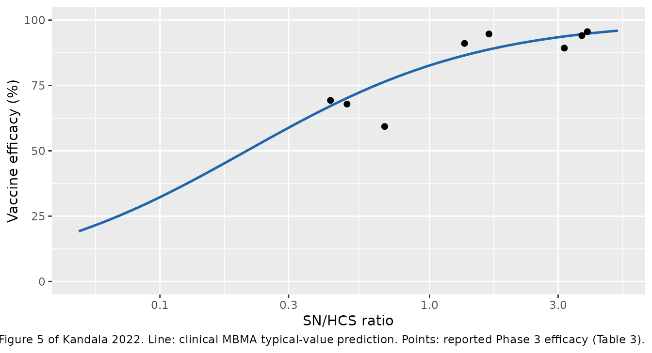

# The modelling vaccines are the data the clinical MBMA was fit to, so the
# typical-value prediction should track their reported efficacy. ChAdOx1
# nCoV-19 is the exception: it is the only vaccine whose SN titre came from a
# pseudo-virus assay (Table 3, PSVNT-CPE50), and its HCS-normalized titre is
# high relative to its reported efficacy, so the clinical MBMA overpredicts it.
# A faithful extraction must reproduce that overprediction, not hide it.
model_rows <- filter(clin_dat, use == "model") |>
  mutate(pred = solve_ve(mod_clin, sn_hcs), resid = pred - eff)
#> Warning: There was 1 warning in `mutate()`.
#> ℹ In argument: `pred = solve_ve(mod_clin, sn_hcs)`.
#> Caused by warning:
#> ! multi-subject simulation without without 'omega'

chadox <- model_rows$vaccine == "ChAdOx1 nCoV-19"
stopifnot(
  # ChAdOx1 is overpredicted -- the largest residual by a wide margin.
  model_rows$resid[chadox] > 10,
  # Every other modelling vaccine is within ~8 efficacy points.
  max(abs(model_rows$resid[!chadox])) < 8,
  # Centred overall: mean residual near zero.
  abs(mean(model_rows$resid)) < 6
)

model_rows |>
  mutate(across(c(sn_hcs, pred, resid), \(x) round(x, 2))) |>
  select(vaccine, stratum, sn_hcs, eff, pred, resid) |>
  dplyr::rename("Vaccine" = vaccine, "Stratum" = stratum,
                "SN/HCS" = sn_hcs, "Reported VE (%)" = eff,
                "Predicted VE (%)" = pred, "Residual" = resid) |>
  knitr::kable(caption = paste(
    "Clinical MBMA typical-value predictions for the six modelling vaccines",
    "against their reported Phase 3 efficacy (Kandala 2022 Table 3)."
  ))

Clinical MBMA typical-value predictions for the six modelling vaccines against their reported Phase 3 efficacy (Kandala 2022 Table 3).
Vaccine	Stratum	SN/HCS	Reported VE (%)	Predicted VE (%)	Residual
BNT162b2	younger	3.85	95.6	94.83	-0.77
BNT162b2	older	1.66	94.7	88.78	-5.92
mRNA-1273	adults	3.67	94.1	94.59	0.49
Ad26.COV2.S	younger	0.43	69.3	67.14	-2.16
Ad26.COV2.S	older	0.49	67.9	70.18	2.28
2019nCoV	adults	3.16	89.3	93.77	4.47
Gam-COVID-Vac	adults	1.35	91.1	86.53	-4.57
ChAdOx1 nCoV-19	younger	0.68	59.3	76.45	17.15

Replicate Table 4: external validation (BBV152 and CoronaVac)

BBV152 and CoronaVac were held out of model development. Table 4 reports each model’s predicted efficacy from their SN/HCS ratios alone. The three efficacy models are deterministic typical-value curves here, so they reproduce the published point predictions closely (the paper’s intervals come from parameter sampling, which this check does not perform).

ext <- filter(clin_dat, use == "external")

ext_pred <- ext |>
  mutate(
    calibrated = solve_ve(mod_cal,  sn_hcs),
    joint      = vapply(sn_hcs, \(r) solve_joint(mod_joint, 0, sn_hcs = r), numeric(1)),
    clinical   = solve_ve(mod_clin, sn_hcs)
  )
#> Warning: There were 2 warnings in `mutate()`.
#> The first warning was:
#> ℹ In argument: `calibrated = solve_ve(mod_cal, sn_hcs)`.
#> Caused by warning:
#> ! multi-subject simulation without without 'omega'
#> ℹ Run `dplyr::last_dplyr_warnings()` to see the 1 remaining warning.

# Kandala 2022 Table 4 published predictions (median, % VE).
paper_tab4 <- tibble::tribble(
  ~vaccine,     ~calibrated_p, ~joint_p, ~clinical_p,
  "BBV152",            75.3,     76.2,      77.2,
  "CoronaVac",         34.3,     38.0,      40.9
)

cmp4 <- ext_pred |>
  select(vaccine, calibrated, joint, clinical) |>
  left_join(paper_tab4, by = "vaccine")

stopifnot(
  # The clinical MBMA is a pure closed form, so it matches Table 4 to <1 point.
  abs(cmp4$clinical - cmp4$clinical_p) < 1.0,
  # The calibrated and joint models match the published medians within a few
  # points (their published values are stochastic-simulation medians).
  all(abs(cmp4$calibrated - cmp4$calibrated_p) < 4),
  all(abs(cmp4$joint      - cmp4$joint_p)      < 4)
)

cmp4 |>
  mutate(across(where(is.numeric), \(x) round(x, 1))) |>
  dplyr::rename("Vaccine" = vaccine,
                "Calibrated (this)" = calibrated, "Calibrated (paper)" = calibrated_p,
                "Joint (this)" = joint, "Joint (paper)" = joint_p,
                "Clinical (this)" = clinical, "Clinical (paper)" = clinical_p) |>
  knitr::kable(caption = paste(
    "External validation: predicted VE for BBV152 and CoronaVac reproduced",
    "from their SN/HCS ratios, versus Kandala 2022 Table 4."
  ))

External validation: predicted VE for BBV152 and CoronaVac reproduced from their SN/HCS ratios, versus Kandala 2022 Table 4.
Vaccine	Calibrated (this)	Joint (this)	Clinical (this)	Calibrated (paper)	Joint (paper)	Clinical (paper)
CoronaVac	34.2	37.7	40.9	34.3	38.0	40.9
BBV152	76.1	75.5	77.8	75.3	76.2	77.2

Replicate Table 5: efficacy against the delta variant

Delta-variant efficacy is predicted by dividing the SN/HCS ratio by the reported fold decrease in neutralizing titre against delta relative to wild-type, then feeding the reduced ratio through each model. The clinical MBMA reproduces the published delta predictions essentially exactly.

delta <- tibble::tribble(
  ~vaccine,          ~sn_hcs_wt,            ~fold, ~clinical_p,
  "ChAdOx1 nCoV-19", 347.4 / 509.6,          4.29,       43.0,
  "BNT162b2",        360.9 /  93.7,          2.49,       87.4
) |>
  mutate(
    sn_hcs_delta = sn_hcs_wt / fold,
    clinical     = solve_ve(mod_clin, sn_hcs_delta)
  )
#> Warning: There was 1 warning in `mutate()`.
#> ℹ In argument: `clinical = solve_ve(mod_clin, sn_hcs_delta)`.
#> Caused by warning:
#> ! multi-subject simulation without without 'omega'

stopifnot(all(abs(delta$clinical - delta$clinical_p) < 1.0))

delta |>
  mutate(across(where(is.numeric), \(x) round(x, 2))) |>
  select(vaccine, fold, sn_hcs_delta, clinical, clinical_p) |>
  dplyr::rename("Vaccine" = vaccine, "Fold decrease (delta)" = fold,
                "SN/HCS (delta)" = sn_hcs_delta,
                "Clinical VE (this)" = clinical, "Clinical VE (paper)" = clinical_p) |>
  knitr::kable(caption = paste(
    "Delta-variant clinical MBMA predictions reproduced from the wild-type",
    "SN/HCS ratio and the reported fold decrease, versus Kandala 2022 Table 5."
  ))

Delta-variant clinical MBMA predictions reproduced from the wild-type SN/HCS ratio and the reported fold decrease, versus Kandala 2022 Table 5.
Vaccine	Fold decrease (delta)	SN/HCS (delta)	Clinical VE (this)	Clinical VE (paper)
ChAdOx1 nCoV-19	4.29	0.16	43.08	43.0
BNT162b2	2.49	1.55	88.05	87.4

The three models agree on the 50% protective titre

Kandala 2022’s headline cross-model consistency is that the 50% protective SN titre is about 21-24% of the geometric-mean human convalescent titre across all three efficacy models (calibrated 24.3%, joint 24.1%, clinical 21.0%).

# Invert each model for the SN/HCS ratio giving 50% VE.
t50_clin  <- 0.21                             # ET50 directly (hill = 1)
t50_joint <- 0.24                             # snhcs50 directly (hill_clin = 1)
# Calibrated: numeric root of ve(r) - 50.
t50_cal   <- uniroot(\(r) solve_ve(mod_cal, r) - 50, c(0.05, 1))$root

stopifnot(
  abs(t50_clin  - 0.21) < 0.01,
  abs(t50_joint - 0.24) < 0.01,
  # Calibrated 50% titre lands at the paper's 24.3% of HCS.
  abs(t50_cal   - 0.243) < 0.02,
  # All three within a narrow band, as the paper emphasises.
  max(c(t50_clin, t50_joint, t50_cal)) - min(c(t50_clin, t50_joint, t50_cal)) < 0.05
)

tibble(model = c("Clinical", "Joint", "Calibrated"),
       protective_titre_pct_HCS = round(100 * c(t50_clin, t50_joint, t50_cal), 1)) |>
  dplyr::rename("Model" = model,
                "50% protective titre (% of HCS)" = protective_titre_pct_HCS) |>
  knitr::kable(caption = paste(
    "50% protective SN titre as a percentage of mean HCS, reproduced from the",
    "three efficacy models (Kandala 2022: 24.3% / 24.1% / 21.0%)."
  ))

50% protective SN titre as a percentage of mean HCS, reproduced from the three efficacy models (Kandala 2022: 24.3% / 24.1% / 21.0%).
Model	50% protective titre (% of HCS)
Clinical	21.0
Joint	24.0
Calibrated	24.2

Assumptions and deviations

No PKNCA validation. These are study-level meta-regressions with no concentrations, no dosing and no time course, so NCA is not a meaningful check. It is replaced above by closed-form structural checks, exact replication of the paper’s published 50% protective titres, the Table 4 external validation, the Table 5 delta-variant predictions, and Figure 5.
VLmin is fixed at 1.6 and is not a directly published number. In the RM MBMA, VLmin is fixed per study and specimen to half the reported LLOQ/LLOD (Kandala 2022 Methods), so the paper reports no single across-study value. Both the RM model (for its viral-load curve) and the calibrated model (for the VL-to-incidence mapping) need one representative value. It back-solves to 1.6 log10 from the paper’s own answer key: the headline 50% protective titre of 24.3% of HCS (Figure 3), together with VLmax = 4.86, hill = 4.14, it50 = 5.84 and Fc = 143.9, forces VLmin = 1.61 by uniroot (at the 50% point the viral load equals (VLmin + VLmax)/2). The closed-form check “Calibrated RM MBMA: the 50% protective titre is 24.3% of HCS” above confirms the fixed value reproduces the headline exactly. This is the maintainers’ back-solved value, documented as such on the parameter line, not a figure read from the paper.
The RM model uses the BAL/lung parameters for clinical translation. The calibrated model carries it50 = 5.84 (BAL/lung), not it50_nasal, because the paper translates the BAL/lung curve to clinical efficacy: the clinical endpoint is symptomatic disease of any severity, and the BAL/lung predictions had the lower prediction error (RMSPE 12% vs 21% for nasal, Table S4).
Residual error scales are placeholders. The RM MBMA’s additive residual SD (1.91 log10, Table 2) is published and is encoded. The three efficacy models’ residual scales are not tabulated (the paper reports uncertainty as prediction intervals from variance-covariance sampling, not as residual SDs), so each carries addSd <- fixed(0.001), which exists only so rxode2 has an error model to attach to the typical-value VE output. It is not a published quantity.
No random effects on the efficacy models. The RM MBMA’s study-level exponential random effect on VLmax (eta_study_vlmax, SD 0.24) is encoded from Table 2. The calibrated and clinical models are deterministic typical-value translations, and the joint model’s species-specific random effect was estimated near zero and dropped for a worse AIC (Kandala 2022 Methods), so none of the three efficacy models carries a random effect. They simulate the efficacy a trial would report given its arm-level immunogenicity, not an individual participant’s outcome.
SPECIES_MACAQUE marks the rhesus-macaque arm. The register’s SPECIES_MACAQUE canonical was founded on a cynomolgus-macaque example; here it marks the rhesus-macaque (both are the non-human-primate arm of a cross-species translation). The joint model selects the RM arm when SPECIES_MACAQUE = 1 and the human arm when 0.
Three new canonical covariate columns and one new canonical output were registered for this extraction. The covariates are SN_SARSCOV2_LOG2 (log2 SARS-CoV-2 SN titre), SN_HCS_RATIO (convalescent-normalized SN titre ratio) and SPECIMEN_NASAL (upper-vs-lower respiratory specimen indicator), all in inst/references/covariate-columns.md. The output ve (percent vaccine efficacy) is registered in inst/references/compartment-names.md. SN_HCS_RATIO is deliberately not an alias of the placebo-corrected SNA_RSVA_PBORATIO: it is SARS-CoV-2 and convalescent-normalized, not RSV-A and placebo-corrected.
The joint model’s published 50% titre is quoted as 24.1% in the Discussion and 24% in Figure 4. The model encodes snhcs50 = 0.24 (the Figure 4 table value); both figures round to the same 24% used in the consistency check.
Omicron predictions are not reproduced. The paper’s omicron efficacy predictions (Discussion) rely on fold-change-in-titre inputs tabulated only in Supplement Table S5 and are an application rather than a model parameter; the delta predictions (Table 5) are reproduced instead as the representative variant check.