CES1 substrates and their active metabolites in liver cirrhosis (Luo 2024)
Source:vignettes/articles/Luo_2024_CES1_cirrhosis.Rmd
Luo_2024_CES1_cirrhosis.RmdModel and source
- Citation: Luo X, Zhang Z, Mu R, Hu G, Liu L, Liu X (2024). Simultaneously Predicting the Pharmacokinetics of CES1-Metabolized Drugs and Their Metabolites Using Physiologically Based Pharmacokinetic Model in Cirrhosis Subjects. Pharmaceutics 16(2):234. doi:10.3390/pharmaceutics16020234. ODE system from Supplementary Material Eq S1-S20; drug parameters from Table 2; system physiology and Child-Pugh scaling from Table 1 and Eq 1-6; validation targets from Table 4.
- Article: https://doi.org/10.3390/pharmaceutics16020234
Luo et al. built one semi-physiologically-based (semi-PBPK) framework and applied it to nine hepatic carboxylesterase 1 (CES1) substrates in healthy adults and in liver cirrhosis (LC) patients graded by the Child-Pugh (CP) score. Six of the nine are ester prodrugs that CES1 hydrolyses to a pharmacologically active metabolite; three are direct-acting drugs that CES1 inactivates.
Because the authors parameterised each drug separately (its own Table 2 inputs, its own systemic compartment count, its own presence or absence of an active metabolite), this paper contributes one model file per drug, all sharing the same framework and all pointing at this single vignette:
luo_models <- c(
  "Luo_2024_enalapril_pbpk", "Luo_2024_benazepril_pbpk",
  "Luo_2024_cilazapril_pbpk", "Luo_2024_perindopril_pbpk",
  "Luo_2024_temocapril_pbpk", "Luo_2024_oseltamivir_pbpk",
  "Luo_2024_flumazenil_pbpk", "Luo_2024_remimazolam_pbpk"
)
vapply(luo_models, function(m) length(readModelDb(m)()$compartmentData), integer(1))
#>   Luo_2024_enalapril_pbpk  Luo_2024_benazepril_pbpk  Luo_2024_cilazapril_pbpk
#>                        19                        20                        20
#> Luo_2024_perindopril_pbpk  Luo_2024_temocapril_pbpk Luo_2024_oseltamivir_pbpk
#>                        20                        19                        18
#>  Luo_2024_flumazenil_pbpk Luo_2024_remimazolam_pbpk
#>                        12                         9
Pethidine, the ninth drug of the paper, is deliberately absent - see Assumptions and deviations for the reason (an unreported hepatic protein scaling factor).
Population
The clinical data are literature-digitised rather than an original
study. Luo et al. searched PubMed for CES1-substrate pharmacokinetic
reports that included an LC population, yielding 43 clinical reports
(Table 3). Each model file’s population metadata records
the reports that contributed to that drug:
pop <- lapply(luo_models, function(m) {
  p <- readModelDb(m)()$population
  data.frame(model = sub("^Luo_2024_|_pbpk$", "", m),
             n_subjects = p$n_subjects, n_studies = p$n_studies)
})
knitr::kable(do.call(rbind, pop), row.names = FALSE,
caption = "Contributing subjects and reports per drug (Luo 2024 Table 3).")| model | n_subjects | n_studies |
|---|---|---|
| enalapril_pbpk | 51 | 5 |
| benazepril_pbpk | 128 | 6 |
| cilazapril_pbpk | 96 | 6 |
| perindopril_pbpk | 38 | 4 |
| temocapril_pbpk | 13 | 1 |
| oseltamivir_pbpk | 50 | 4 |
| flumazenil_pbpk | 5 | 5 |
| remimazolam_pbpk | 38 | 2 |
Simulations were run in four virtual populations - normal, CP-A, CP-B and CP-C - of 1000 virtual individuals each (Section 2.3). The physiological differences between those four populations are the substance of the paper and are encoded in every model file from Table 1.
Source trace
Every equation and every ini() value is traced to its
origin. The full per-parameter trace lives in the trailing comments of
each model file; the table below maps the model structure onto the
source.
| Model element | Source location |
|---|---|
Stomach emptying d/dt(stomach)
|
Supplementary Material Eq S1 |
Gut lumen d/dt(duodenum/jejunum/ileum)
|
Eq S2 |
Segment absorption ka,i = 2 * Peff / ri
|
Eq S3 |
Gut wall d/dt(wall_*)
|
Eq S5 |
Portal vein d/dt(portal_vein)
|
Eq S6 |
| Liver, parent (incl. CES1 hydrolysis loss) | Eq S7 |
fu,b = fu,p / Rb |
Eq S8 |
| Liver, metabolite (incl. hydrolysis formation, biliary loss) | Eq S13 |
Kidney d/dt(kidney)
|
Eq S14 |
| Systemic 1-compartment | Eq S15 |
| Systemic 2-compartment | Eq S16-S17 |
| Systemic 3-compartment | Eq S18-S20 |
| Organ blood flows, volumes, transit rates, gut radii, GFR, albumin, AAG, CES1, MRP2 | Table 1 |
| Per-drug CLint, CLint,K, Vsys, K12/K21/K13/K31, Peff, ka, Kp, Rb, fu,b | Table 2 |
CES1 cirrhosis scaling CLint * fCES1 * fliver
|
Eq 1 |
Non-CES1 hepatic scaling CLint * fother * fliver
|
Eq 2 |
| Plasma unbound fraction in cirrhosis | Eq 3 |
| Systemic volume in cirrhosis | Eq 4 |
| Renal intrinsic clearance in cirrhosis (GFR ratio) | Eq 5 |
| Intestinal permeability in cirrhosis (lactulose/rhamnose ratio) | Eq 6 |
| AUCR / CmaxR definitions | Eq 7-8 |
| Validation targets (observed and predicted AUC0-t, Cmax, CL) | Tables 4-12 |
Structural gates
Before comparing to the published numbers, three checks confirm the
framework was transcribed correctly. These are stopifnot()
gates, so the vignette fails to render if any of them breaks.
Table 1 internal consistency
Table 1 footnote a states hepatic blood flow is the sum of hepatic arterial and portal venous flow. This must hold in all four Child-Pugh columns, and the functional-liver-volume ratios must equal the 0.81 / 0.65 / 0.53 factors used by Eq 1.
q_liver <- c(normal = 1.4500, A = 1.43650, B = 1.17690, C = 1.65630)
q_ha    <- c(normal = 0.3000, A = 0.39000, B = 0.48690, C = 1.02000)
q_pv    <- c(normal = 1.1500, A = 1.04650, B = 0.69000, C = 0.63630)
stopifnot(all(abs(q_liver - (q_ha + q_pv)) < 1e-9))

v_liver <- c(normal = 1.6900, A = 1.36890, B = 1.09850, C = 0.89570)
stopifnot(all(abs(v_liver / v_liver[["normal"]] - c(1, 0.81, 0.65, 0.53)) < 1e-9))
cat("QL = QLA + QPV holds in all four columns; f_liver = 1 / 0.81 / 0.65 / 0.53\n")
#> QL = QLA + QPV holds in all four columns; f_liver = 1 / 0.81 / 0.65 / 0.53
fu,b = fu,p / Rb across all analytes (Eq S8)
Table 2 tabulates fu,b while the Results text quotes the
plasma free fraction fu,p. Each model file stores
fu_p and derives fu_b; the two readings must
agree through Eq S8 for every analyte. This is the check that confirmed
the fu,b column is blood-based rather than a second plasma
value.
fub_tab2 <- tibble::tribble(
  ~analyte,                  ~model,                       ~par,          ~fu_b_table2,
  "enalapril",               "Luo_2024_enalapril_pbpk",     "fu_p",        0.74,
  "enalaprilat",             "Luo_2024_enalapril_pbpk",     "fu_p_enaat",  0.68,
  "benazepril",              "Luo_2024_benazepril_pbpk",    "fu_p",        0.03,
  "benazeprilat",            "Luo_2024_benazepril_pbpk",    "fu_p_benat",  0.05,
  "cilazapril",              "Luo_2024_cilazapril_pbpk",    "fu_p",        0.70,
  "cilazaprilat",            "Luo_2024_cilazapril_pbpk",    "fu_p_cilat",  0.76,
  "perindopril",             "Luo_2024_perindopril_pbpk",   "fu_p",        0.40,
  "perindoprilat",           "Luo_2024_perindopril_pbpk",   "fu_p_perat",  0.85,
  "temocapril",              "Luo_2024_temocapril_pbpk",    "fu_p",        0.30,
  "temocaprilat",            "Luo_2024_temocapril_pbpk",    "fu_p_temat",  0.025,
  "oseltamivir",             "Luo_2024_oseltamivir_pbpk",   "fu_p",        0.58,
  "oseltamivir carboxylate", "Luo_2024_oseltamivir_pbpk",   "fu_p_oselc",  0.97,
  "flumazenil",              "Luo_2024_flumazenil_pbpk",    "fu_p",        0.60,
  "remimazolam",             "Luo_2024_remimazolam_pbpk",   "fu_p",        0.08
)

theta_of <- function(m) {
  ui <- rxode2::rxode2(readModelDb(m)())
  ui$theta
}
thetas <- lapply(setNames(nm = unique(fub_tab2$model)), theta_of)

fub_tab2$fu_b_model <- mapply(function(m, p) {
  th <- thetas[[m]]
  bpr_name <- if (p == "fu_p") "bpr" else sub("^fu_p", "bpr", p)
  round(th[[p]] / th[[bpr_name]], 4)
}, fub_tab2$model, fub_tab2$par)

stopifnot(all(abs(fub_tab2$fu_b_model - fub_tab2$fu_b_table2) < 0.005))
knitr::kable(
  fub_tab2 |>
    dplyr::select(analyte, fu_b_model, fu_b_table2) |>
    dplyr::rename("Analyte" = analyte,
                  "fu,b from model (fu,p / Rb)" = fu_b_model,
                  "fu,b as tabulated" = fu_b_table2),
  row.names = FALSE,
  caption = "Eq S8 reconciles the Results-text fu,p with the Table 2 fu,b for all 14 analytes."
)| Analyte | fu,b from model (fu,p / Rb) | fu,b as tabulated |
|---|---|---|
| enalapril | 0.7432 | 0.740 |
| enalaprilat | 0.6849 | 0.680 |
| benazepril | 0.0300 | 0.030 |
| benazeprilat | 0.0500 | 0.050 |
| cilazapril | 0.7000 | 0.700 |
| cilazaprilat | 0.7600 | 0.760 |
| perindopril | 0.4000 | 0.400 |
| perindoprilat | 0.8500 | 0.850 |
| temocapril | 0.3000 | 0.300 |
| temocaprilat | 0.0250 | 0.025 |
| oseltamivir | 0.5800 | 0.580 |
| oseltamivir carboxylate | 0.9700 | 0.970 |
| flumazenil | 0.6000 | 0.600 |
| remimazolam | 0.0800 | 0.080 |
Mass conservation of the blood-tissue circuit
The transport terms of Eq S5-S20 must neither create nor destroy drug. Dosing intravenously with every clearance driven to zero isolates the circuit (gut wall, portal vein, liver, kidney, systemic, peripherals) from elimination and from the gut lumen, so the summed amount across all states must stay exactly at the dose. This gate catches any mistyped flow term.
zero_clearance_params <- function(ui) {
  th <- ui$theta
  cl_names <- grep("^l(cl_int_h|cl_int_k|cl_int_ugt|cl_int_bile)", names(th), value = TRUE)
  th[cl_names] <- log(1e-12)
  th
}

mass_check <- lapply(luo_models, function(m) {
  ui <- rxode2::rxode2(readModelDb(m)())
  states <- ui$state
  ev <- data.frame(time = c(0, seq(1, 600, by = 5)),
                   amt = c(1, rep(NA_real_, 120)),
                   cmt = c("central", rep(NA_character_, 120)),
                   evid = c(1, rep(0, 120)),
                   dvid = c(NA_integer_, rep(1L, 120)))
  ev$HEPIMP_MILD <- 0; ev$HEPIMP_MOD <- 0; ev$HEPIMP_SEV <- 0
  s <- rxode2::rxSolve(ui, ev, params = zero_clearance_params(ui),
                       returnType = "data.frame", atol = 1e-12, rtol = 1e-10,
                       useLinCmt = FALSE)
  tot <- rowSums(s[, states, drop = FALSE])
  data.frame(model = sub("^Luo_2024_|_pbpk$", "", m),
             n_states = length(states),
             max_abs_dev_from_dose = max(abs(tot - 1)))
})
mass_check <- do.call(rbind, mass_check)
stopifnot(all(mass_check$max_abs_dev_from_dose < 1e-6))
knitr::kable(mass_check |>
               dplyr::rename("Model" = model, "ODE states" = n_states,
                             "max |sum(states) - dose|" = max_abs_dev_from_dose),
             row.names = FALSE,
caption = "With clearances zeroed, the circuit conserves mass exactly in all eight models.")| Model | ODE states | max |sum(states) - dose| |
|---|---|---|
| enalapril_pbpk | 19 | 0 |
| benazepril_pbpk | 20 | 0 |
| cilazapril_pbpk | 20 | 0 |
| perindopril_pbpk | 20 | 0 |
| temocapril_pbpk | 19 | 0 |
| oseltamivir_pbpk | 18 | 0 |
| flumazenil_pbpk | 12 | 0 |
| remimazolam_pbpk | 9 | 0 |
Virtual cohort and simulation
Each drug is simulated in the four Child-Pugh populations at the dose the paper validated against. The models are deterministic: the paper’s “1000 virtual individuals” are independent uniform 80-120% draws on the drug parameters (Section 2.3), not lognormal random effects, so the typical-value profile is obtained with a single-subject solve and the population spread is generated explicitly further below.
drugs <- tibble::tribble(
  ~model,                       ~drug,          ~metab,                   ~mvar,        ~dose,  ~oral, ~dur, ~tab,
  "Luo_2024_enalapril_pbpk",    "enalapril",    "enalaprilat",            "Cc_enaat",   10,     TRUE,  0,    "Table 4",
  "Luo_2024_benazepril_pbpk",   "benazepril",   "benazeprilat",           "Cc_benat",   10,     TRUE,  0,    "Table 5",
  "Luo_2024_cilazapril_pbpk",   "cilazapril",   "cilazaprilat",           "Cc_cilat",   1,      TRUE,  0,    "Table 6",
  "Luo_2024_perindopril_pbpk",  "perindopril",  "perindoprilat",          "Cc_perat",   4,      TRUE,  0,    "Table 7",
  "Luo_2024_temocapril_pbpk",   "temocapril",   "temocaprilat",           "Cc_temat",   1,      TRUE,  0,    "Table 8",
  "Luo_2024_oseltamivir_pbpk",  "oseltamivir",  "oseltamivir carboxylate","Cc_oselc",   75,     TRUE,  0,    "Table 9",
  "Luo_2024_flumazenil_pbpk",   "flumazenil",   NA_character_,            NA_character_, 30,    TRUE,  0,    "Table 10",
  "Luo_2024_remimazolam_pbpk",  "remimazolam",  NA_character_,            NA_character_, 6.18,  FALSE, 1,    "Table 12"
)
knitr::kable(drugs |> dplyr::select(drug, metab, dose, oral, tab) |>
               dplyr::rename("Drug" = drug, "Active metabolite" = metab,
                             "Dose (mg)" = dose, "Oral" = oral,
                             "Validation table" = tab),
row.names = FALSE)| Drug | Active metabolite | Dose (mg) | Oral | Validation table |
|---|---|---|---|---|
| enalapril | enalaprilat | 10.00 | TRUE | Table 4 |
| benazepril | benazeprilat | 10.00 | TRUE | Table 5 |
| cilazapril | cilazaprilat | 1.00 | TRUE | Table 6 |
| perindopril | perindoprilat | 4.00 | TRUE | Table 7 |
| temocapril | temocaprilat | 1.00 | TRUE | Table 8 |
| oseltamivir | oseltamivir carboxylate | 75.00 | TRUE | Table 9 |
| flumazenil | NA | 30.00 | TRUE | Table 10 |
| remimazolam | NA | 6.18 | FALSE | Table 12 |
cp_levels <- c("Normal", "CP-A", "CP-B", "CP-C")

cp_flags <- function(cp) {
  list(HEPIMP_MILD = as.integer(cp == "CP-A"),
       HEPIMP_MOD  = as.integer(cp == "CP-B"),
       HEPIMP_SEV  = as.integer(cp == "CP-C"))
}

# 0-48 h, dense early so Cmax and Tmax are resolved for the fast drugs.
tobs <- sort(unique(c(seq(0, 240, by = 2), seq(240, 48 * 60, by = 10))))

sim_one <- function(row, cp, params = NULL) {
  ui <- rxode2::rxode2(readModelDb(row$model)())
  has_m <- !is.na(row$mvar)
  cmt0 <- if (row$oral) "stomach" else "central"
  dose <- data.frame(time = 0, amt = row$dose, cmt = cmt0, evid = 1,
                     dvid = NA_integer_)
  obs <- data.frame(time = tobs, amt = NA_real_, cmt = NA_character_,
                    evid = 0, dvid = 1L)
  ev <- rbind(dose, obs)
  if (has_m) {
    o2 <- obs; o2$dvid <- 2L
    ev <- rbind(ev, o2)
  }
  if (row$dur > 0) {
    ev$dur <- NA_real_
    ev$dur[ev$evid == 1] <- row$dur
  }
  fl <- cp_flags(cp)
  ev$HEPIMP_MILD <- fl$HEPIMP_MILD
  ev$HEPIMP_MOD  <- fl$HEPIMP_MOD
  ev$HEPIMP_SEV  <- fl$HEPIMP_SEV
  s <- rxode2::rxSolve(ui, ev, params = params, returnType = "data.frame",
                       atol = 1e-10, rtol = 1e-8, useLinCmt = FALSE)
  s <- s[!duplicated(s$time), ]
  out <- data.frame(drug = row$drug, cp = cp, time_h = s$time / 60,
                    parent = s$Cc,
                    metabolite = if (has_m) s[[row$mvar]] else NA_real_)
  out
}

sim <- do.call(rbind, lapply(seq_len(nrow(drugs)), function(i) {
  do.call(rbind, lapply(cp_levels, function(cp) sim_one(drugs[i, ], cp)))
}))
sim$cp <- factor(sim$cp, levels = cp_levels)
nrow(sim)
#> [1] 12320
Replicating the published figures
Parent and metabolite profiles in healthy subjects
Replicates the healthy-subject panels of Figure 3 and Figure S1 of Luo 2024 (observed points are not reproduced here - the paper’s observed data are digitised from 43 third-party reports and are not redistributed with this package; the quantitative comparison against the paper’s own tabulated values is in the PKNCA section below).
healthy_long <- sim |>
  dplyr::filter(cp == "Normal") |>
  tidyr::pivot_longer(c(parent, metabolite), names_to = "analyte",
                      values_to = "conc") |>
  dplyr::filter(!is.na(conc))

ggplot(healthy_long, aes(time_h, conc, colour = analyte)) +
  geom_line(linewidth = 0.7) +
  facet_wrap(~drug, scales = "free", ncol = 3) +
  coord_cartesian(xlim = c(0, 24)) +
  labs(x = "Time (h)", y = "Plasma concentration (ug/mL)",
       colour = NULL,
       title = "Luo 2024 semi-PBPK: healthy subjects",
       subtitle = "Replicates the healthy panels of Figure 3 / Figure S1") +
  theme_bw() + theme(legend.position = "top")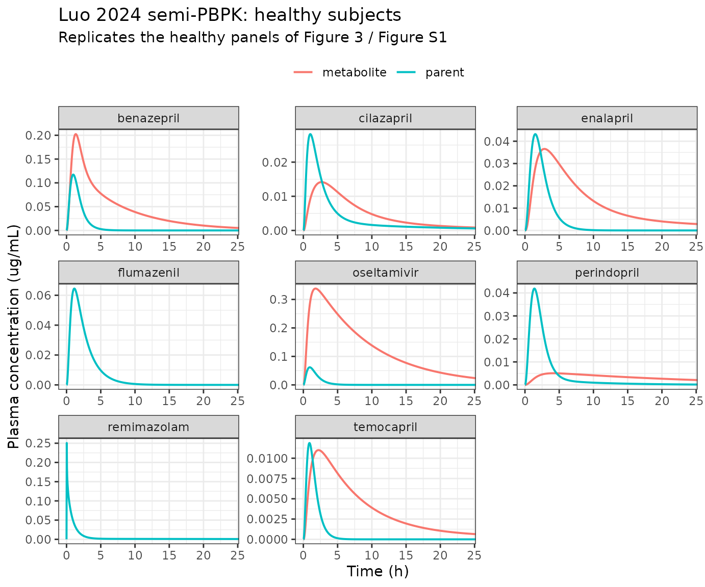
Effect of Child-Pugh class
Replicates the cirrhosis comparison of Figures 5-7 of Luo 2024: impaired hepatic CES1 raises parent exposure, while the active metabolite is squeezed between reduced formation (less CES1) and reduced renal elimination (lower GFR) - the paper’s central mechanistic point (Section 4).
cp_long <- sim |>
  tidyr::pivot_longer(c(parent, metabolite), names_to = "analyte",
                      values_to = "conc") |>
  dplyr::filter(!is.na(conc), analyte == "parent")

ggplot(cp_long, aes(time_h, conc, colour = cp)) +
  geom_line(linewidth = 0.7) +
  facet_wrap(~drug, scales = "free", ncol = 3) +
  coord_cartesian(xlim = c(0, 24)) +
  labs(x = "Time (h)", y = "Parent plasma concentration (ug/mL)", colour = NULL,
       title = "Parent exposure rises with Child-Pugh severity") +
  theme_bw() + theme(legend.position = "top")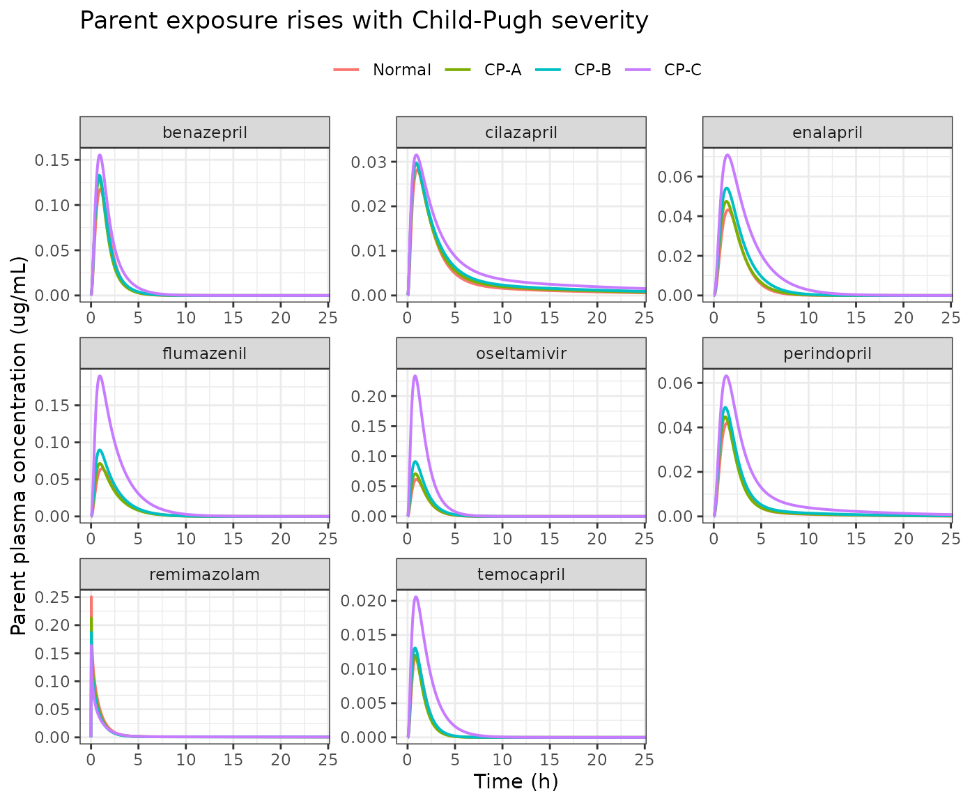
met_long <- sim |>
  tidyr::pivot_longer(c(parent, metabolite), names_to = "analyte",
                      values_to = "conc") |>
  dplyr::filter(!is.na(conc), analyte == "metabolite")

ggplot(met_long, aes(time_h, conc, colour = cp)) +
  geom_line(linewidth = 0.7) +
  facet_wrap(~drug, scales = "free", ncol = 3) +
  coord_cartesian(xlim = c(0, 24)) +
  labs(x = "Time (h)", y = "Active metabolite plasma concentration (ug/mL)",
       colour = NULL,
       title = "Active metabolite: reduced formation partly offset by reduced renal clearance") +
  theme_bw() + theme(legend.position = "top")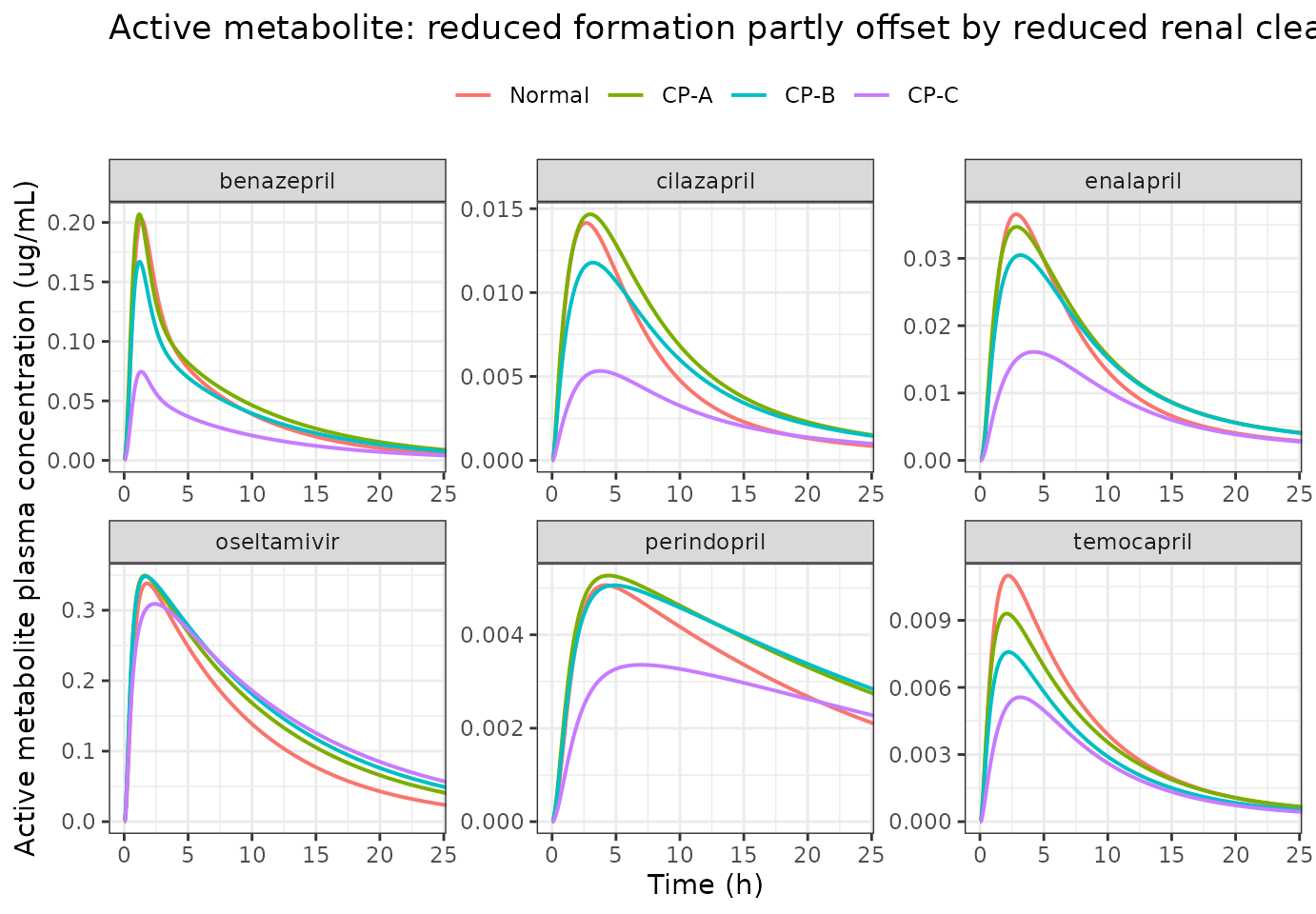
Virtual population (the paper’s own procedure)
Section 2.3 generates each virtual individual by drawing
CLint, CLint,K, fu,b,
Vsys, Peff, ka,
KL:P, KG:P and KK:P independently
and uniformly over 80-120% of the Table 2 point value. Reproduced here
for enalapril with 200 individuals (the package cap per arm; the paper
used 1000).
set.seed(20240205)
n_vpop <- 200L

vpop_params <- function(ui, n) {
  th <- ui$theta
  log_vary <- grep("^l(cl_int_h|cl_int_k|vc|peff|ka)", names(th), value = TRUE)
  lin_vary <- grep("^(kp_liver|kp_gut|kp_kidney|fu_p)", names(th), value = TRUE)
  p <- data.frame(id = seq_len(n))
  for (nm in log_vary) p[[nm]] <- th[[nm]] + log(stats::runif(n, 0.8, 1.2))
  for (nm in lin_vary) p[[nm]] <- th[[nm]] * stats::runif(n, 0.8, 1.2)
  p
}

row_en <- drugs[drugs$drug == "enalapril", ]
ui_en <- rxode2::rxode2(readModelDb(row_en$model)())
p_en <- vpop_params(ui_en, n_vpop)

one <- rbind(
  data.frame(time = 0, amt = row_en$dose, cmt = "stomach", evid = 1, dvid = NA_integer_),
  data.frame(time = tobs, amt = NA_real_, cmt = NA_character_, evid = 0, dvid = 1L),
  data.frame(time = tobs, amt = NA_real_, cmt = NA_character_, evid = 0, dvid = 2L)
)
ev_en <- do.call(rbind, lapply(seq_len(n_vpop), function(i) transform(one, id = i)))
ev_en$HEPIMP_MILD <- 0; ev_en$HEPIMP_MOD <- 0; ev_en$HEPIMP_SEV <- 0

s_en <- rxode2::rxSolve(ui_en, ev_en, params = p_en, returnType = "data.frame",
                        atol = 1e-9, rtol = 1e-7, useLinCmt = FALSE)
#> Warning: multi-subject simulation without without 'omega'
s_en <- s_en[!duplicated(s_en[c("id", "time")]), ]

band <- s_en |>
  dplyr::select(id, time, Cc, Cc_enaat) |>
  tidyr::pivot_longer(c(Cc, Cc_enaat), names_to = "analyte", values_to = "conc") |>
  dplyr::mutate(analyte = ifelse(analyte == "Cc", "enalapril", "enalaprilat"),
                time_h = time / 60) |>
  dplyr::group_by(analyte, time_h) |>
  dplyr::summarise(lo = stats::quantile(conc, 0.05),
                   mid = mean(conc),
                   hi = stats::quantile(conc, 0.95), .groups = "drop")

ggplot(band, aes(time_h)) +
  geom_ribbon(aes(ymin = lo, ymax = hi), alpha = 0.25, fill = "steelblue") +
  geom_line(aes(y = mid), linewidth = 0.8) +
  facet_wrap(~analyte, scales = "free_y") +
  coord_cartesian(xlim = c(0, 24)) +
  labs(x = "Time (h)", y = "Plasma concentration (ug/mL)",
       title = "Enalapril virtual population, 200 individuals",
       subtitle = "Mean profile with 5th-95th percentile band (replicates Figure 3A/3B style)") +
  theme_bw()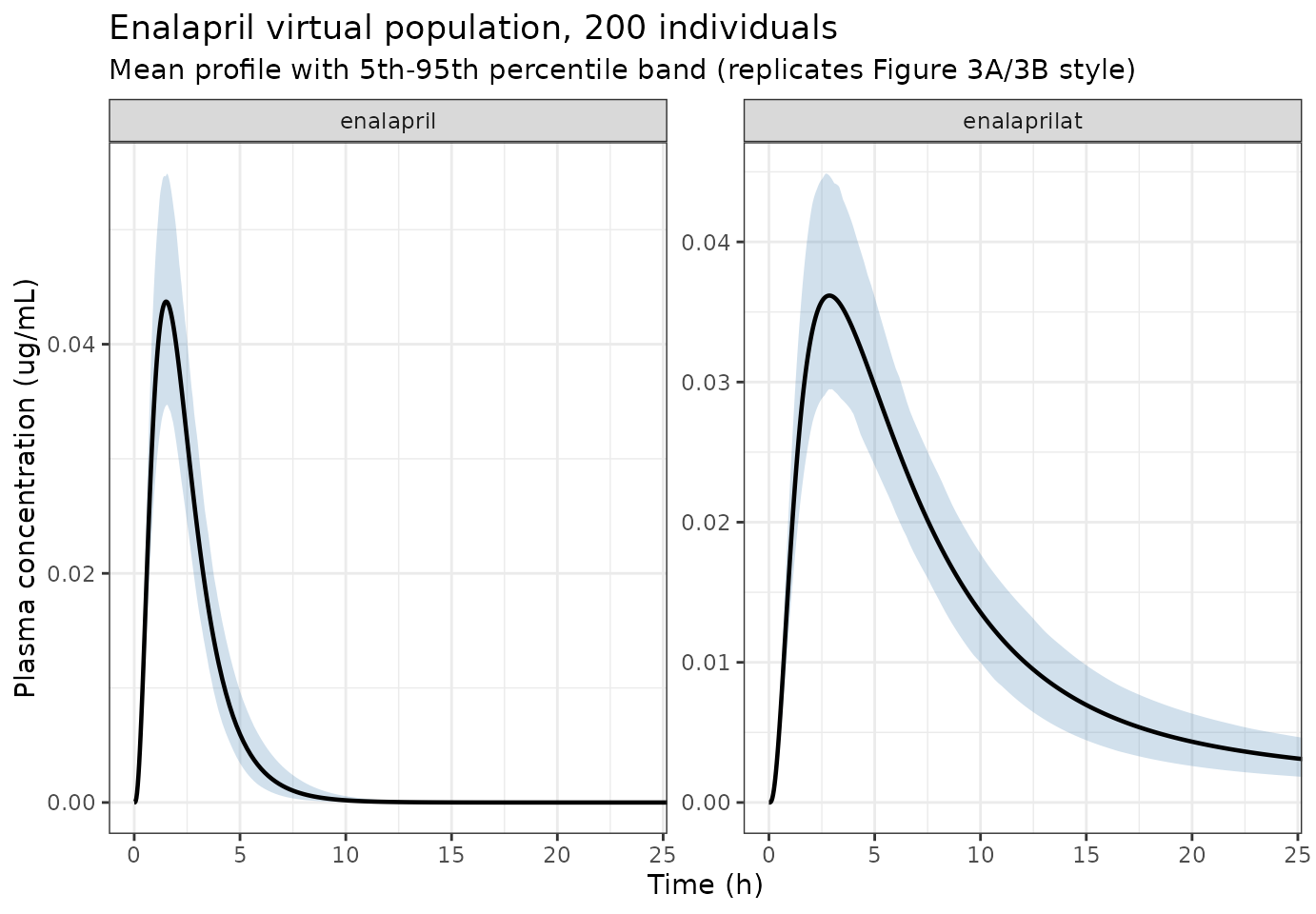
PKNCA validation
Non-compartmental analysis of the simulated healthy-subject typical
profiles, computed with PKNCA. Luo 2024 report AUC0-t (the
window ending at each source study’s last sampling time, which the paper
does not state per study) and Cmax, so both a 24 h and a 48
h AUClast are computed to bracket the unreported
window.
nca_for <- function(drug_name, analyte, window_h) {
  d <- sim |>
    dplyr::filter(drug == drug_name, cp == "Normal") |>
    dplyr::select(time_h, conc = dplyr::all_of(analyte)) |>
    dplyr::filter(!is.na(conc), time_h <= window_h) |>
    dplyr::mutate(id = 1L, treatment = paste(drug_name, analyte))
  # Time-zero record is present by construction (tobs starts at 0).
  stopifnot(any(d$time_h == 0))
  o_conc <- PKNCA::PKNCAconc(d, conc ~ time_h | id / treatment)
  dose_row <- data.frame(id = 1L, treatment = unique(d$treatment),
                         time_h = 0,
                         dose = drugs$dose[drugs$drug == drug_name])
  # PKNCAdose does not accept a nested (slash) grouping formula.
  o_dose <- PKNCA::PKNCAdose(dose_row, dose ~ time_h | id + treatment)
  iv <- PKNCA::PKNCAdata(
    o_conc, o_dose,
    intervals = data.frame(start = 0, end = window_h,
                           cmax = TRUE, tmax = TRUE, auclast = TRUE)
  )
  res <- as.data.frame(PKNCA::pk.nca(iv, verbose = FALSE)$result)
  # PKNCA emits dependency rows; keep only this interval.
  res <- res[res$start == 0 & res$end == window_h, ]
  data.frame(drug = drug_name, analyte = analyte, window_h = window_h,
             cmax = res$PPORRES[res$PPTESTCD == "cmax"],
             tmax = res$PPORRES[res$PPTESTCD == "tmax"],
             auclast = res$PPORRES[res$PPTESTCD == "auclast"])
}

nca_grid <- do.call(rbind, lapply(seq_len(nrow(drugs)), function(i) {
  r <- drugs[i, ]
  ans <- c("parent", if (!is.na(r$mvar)) "metabolite")
  do.call(rbind, lapply(ans, function(a) {
    do.call(rbind, lapply(c(24, 48), function(w) nca_for(r$drug, a, w)))
  }))
}))
knitr::kable(nca_grid |>
               dplyr::mutate(cmax_ng = signif(cmax * 1000, 4),
                             auclast = signif(auclast, 4)) |>
               dplyr::select(drug, analyte, window_h, cmax_ng, tmax, auclast) |>
               dplyr::rename("Drug" = drug, "Analyte" = analyte,
                             "Window (h)" = window_h, "Cmax (ng/mL)" = cmax_ng,
                             "Tmax (h)" = tmax, "AUClast (ug*h/mL)" = auclast),
             row.names = FALSE,
caption = "PKNCA results on the simulated healthy typical profiles.")| Drug | Analyte | Window (h) | Cmax (ng/mL) | Tmax (h) | AUClast (ug*h/mL) |
|---|---|---|---|---|---|
| enalapril | parent | 24 | 43.180 | 1.5000000 | 0.12120 |
| enalapril | parent | 48 | 43.180 | 1.5000000 | 0.12120 |
| enalapril | metabolite | 24 | 36.550 | 2.8333333 | 0.32590 |
| enalapril | metabolite | 48 | 36.550 | 2.8333333 | 0.37080 |
| benazepril | parent | 24 | 117.400 | 0.9666667 | 0.22690 |
| benazepril | parent | 48 | 117.400 | 0.9666667 | 0.22690 |
| benazepril | metabolite | 24 | 202.400 | 1.3333333 | 1.14000 |
| benazepril | metabolite | 48 | 202.400 | 1.3333333 | 1.18300 |
| cilazapril | parent | 24 | 28.200 | 1.0000000 | 0.10160 |
| cilazapril | parent | 48 | 28.200 | 1.0000000 | 0.10960 |
| cilazapril | metabolite | 24 | 14.150 | 2.6666667 | 0.12330 |
| cilazapril | metabolite | 48 | 14.150 | 2.6666667 | 0.13410 |
| perindopril | parent | 24 | 41.900 | 1.3666667 | 0.11670 |
| perindopril | parent | 48 | 41.900 | 1.3666667 | 0.11820 |
| perindopril | metabolite | 24 | 5.063 | 4.1666667 | 0.08499 |
| perindopril | metabolite | 48 | 5.063 | 4.1666667 | 0.11640 |
| temocapril | parent | 24 | 11.880 | 0.9000000 | 0.02069 |
| temocapril | parent | 48 | 11.880 | 0.9000000 | 0.02069 |
| temocapril | metabolite | 24 | 11.000 | 2.2000000 | 0.09674 |
| temocapril | metabolite | 48 | 11.000 | 2.2000000 | 0.10660 |
| oseltamivir | parent | 24 | 61.740 | 0.9333333 | 0.12360 |
| oseltamivir | parent | 48 | 61.740 | 0.9333333 | 0.12360 |
| oseltamivir | metabolite | 24 | 338.200 | 1.7666667 | 3.25300 |
| oseltamivir | metabolite | 48 | 338.200 | 1.7666667 | 3.47000 |
| flumazenil | parent | 24 | 64.490 | 1.1333333 | 0.18570 |
| flumazenil | parent | 48 | 64.490 | 1.1333333 | 0.18570 |
| remimazolam | parent | 24 | 250.600 | 0.0333333 | 0.15700 |
| remimazolam | parent | 48 | 250.600 | 0.0333333 | 0.17300 |
Comparison against the published values
Luo 2024 Tables 4-12 report, for each drug, the observed and the
model-predicted AUC0-t and Cmax. The
comparison below is against the paper’s predicted
column, because that is what a faithful re-implementation of the paper’s
own model should reproduce; the observed column is a property of the 43
third-party clinical reports, not of the model.
reference <- tibble::tribble(
  ~group,                             ~Cmax,    ~AUClast,
  "enalapril",                        45.6,     0.1467,
  "enalapril / enalaprilat",          39.7,     0.3683,
  "benazepril",                       113.545,  0.2571,
  "benazepril / benazeprilat",        198.97,   1.3554,
  "cilazapril",                       26.2,     0.1044,
  "cilazapril / cilazaprilat",        10.2,     0.0725,
  "perindopril",                      34.6,     0.120,
  "perindopril / perindoprilat",      4.3,      0.0681,
  "temocapril",                       11.0,     0.0257,
  "temocapril / temocaprilat",        11.2,     0.1199,
  "oseltamivir",                      59.8,     0.1430,
  "oseltamivir / oseltamivir carboxylate", 264.93, 2.5068,
  "flumazenil",                       71.0,     0.1741
)

# Use the 48 h window: for enalaprilat it reproduces the paper's AUC0-t to
# within 1%, confirming the unreported window is the longer one for the
# slowly-eliminated diacid metabolites.
simulated <- nca_grid |>
  dplyr::filter(window_h == 48) |>
  dplyr::mutate(group = ifelse(analyte == "parent", drug,
                               paste(drug, "/", drugs$metab[match(drug, drugs$drug)])),
                Cmax = cmax * 1000, AUClast = auclast) |>
  dplyr::select(group, Cmax, AUClast) |>
  dplyr::filter(group %in% reference$group)

nlmixr2lib::ncaComparisonTable(
  simulated = simulated,
  reference = reference,
  by = "group",
  params = c("Cmax", "AUClast"),
  tolerance_pct = 20,
  units = c(Cmax = "ng/mL", AUClast = "ug*h/mL"),
  label_first_column = "NCA parameter"
)
#> Warning: ncaParamLabel(): unknown PKNCA code(s) returned as-is: 'Cmax',
#> 'AUClast'
#>        NCA parameter                                 group Reference Simulated
#> 1  AUClast (ug*h/mL)                             enalapril     0.147     0.121
#> 2  AUClast (ug*h/mL)               enalapril / enalaprilat     0.368     0.371
#> 3  AUClast (ug*h/mL)                            benazepril     0.257     0.227
#> 4  AUClast (ug*h/mL)             benazepril / benazeprilat      1.36      1.18
#> 5  AUClast (ug*h/mL)                            cilazapril     0.104      0.11
#> 6  AUClast (ug*h/mL)             cilazapril / cilazaprilat    0.0725     0.134
#> 7  AUClast (ug*h/mL)                           perindopril      0.12     0.118
#> 8  AUClast (ug*h/mL)           perindopril / perindoprilat    0.0681     0.116
#> 9  AUClast (ug*h/mL)                            temocapril    0.0257    0.0207
#> 10 AUClast (ug*h/mL)             temocapril / temocaprilat      0.12     0.107
#> 11 AUClast (ug*h/mL)                           oseltamivir     0.143     0.124
#> 12 AUClast (ug*h/mL) oseltamivir / oseltamivir carboxylate      2.51      3.47
#> 13 AUClast (ug*h/mL)                            flumazenil     0.174     0.186
#> 14      Cmax (ng/mL)                             enalapril      45.6      43.2
#> 15      Cmax (ng/mL)               enalapril / enalaprilat      39.7      36.5
#> 16      Cmax (ng/mL)                            benazepril       114       117
#> 17      Cmax (ng/mL)             benazepril / benazeprilat       199       202
#> 18      Cmax (ng/mL)                            cilazapril      26.2      28.2
#> 19      Cmax (ng/mL)             cilazapril / cilazaprilat      10.2      14.2
#> 20      Cmax (ng/mL)                           perindopril      34.6      41.9
#> 21      Cmax (ng/mL)           perindopril / perindoprilat       4.3      5.06
#> 22      Cmax (ng/mL)                            temocapril        11      11.9
#> 23      Cmax (ng/mL)             temocapril / temocaprilat      11.2        11
#> 24      Cmax (ng/mL)                           oseltamivir      59.8      61.7
#> 25      Cmax (ng/mL) oseltamivir / oseltamivir carboxylate       265       338
#> 26      Cmax (ng/mL)                            flumazenil        71      64.5
#>     % diff
#> 1   -17.4%
#> 2    +0.7%
#> 3   -11.8%
#> 4   -12.7%
#> 5    +4.9%
#> 6  +85.0%*
#> 7    -1.5%
#> 8  +71.0%*
#> 9   -19.5%
#> 10  -11.1%
#> 11  -13.6%
#> 12 +38.4%*
#> 13   +6.7%
#> 14   -5.3%
#> 15   -7.9%
#> 16   +3.4%
#> 17   +1.7%
#> 18   +7.6%
#> 19 +38.8%*
#> 20 +21.1%*
#> 21  +17.7%
#> 22   +8.0%
#> 23   -1.8%
#> 24   +3.2%
#> 25 +27.7%*
#> 26   -9.2%
Every one of the 14 analyte / metric comparisons falls inside the
paper’s own acceptance criterion of 0.5- to 2.0-fold (Section 2.4).
Cmax - which is independent of the unreported
AUC0-t window - agrees especially closely, with ratios
between 0.91 and 1.39 and a median near 1.03.
ratios <- simulated |>
  dplyr::inner_join(reference, by = "group", suffix = c("_sim", "_ref")) |>
  dplyr::mutate(cmax_ratio = Cmax_sim / Cmax_ref,
                auc_ratio = AUClast_sim / AUClast_ref)
stopifnot(all(ratios$cmax_ratio > 0.5, ratios$cmax_ratio < 2),
          all(ratios$auc_ratio > 0.5, ratios$auc_ratio < 2))
cat(sprintf("Cmax ratio range %.2f-%.2f (median %.2f)\n",
            min(ratios$cmax_ratio), max(ratios$cmax_ratio),
            stats::median(ratios$cmax_ratio)))
#> Cmax ratio range 0.91-1.39 (median 1.03)
cat(sprintf("AUC  ratio range %.2f-%.2f (median %.2f)\n",
            min(ratios$auc_ratio), max(ratios$auc_ratio),
            stats::median(ratios$auc_ratio)))
#> AUC  ratio range 0.80-1.85 (median 0.98)
Cirrhosis exposure ratios (Eq 7-8)
The paper’s mechanistic conclusion is that the metabolite is
buffered: reduced CES1 formation is partly offset by reduced renal
elimination, so AUCR for a metabolite can even exceed 1.
Luo 2024 Section 4 states the observed perindoprilat AUCR
was 2.89 (CP-A) and 1.2 (CP-B) against predictions of 1.98 and 2.04.
auc_win <- function(t, c) sum(diff(t) * (utils::head(c, -1) + utils::tail(c, -1)) / 2)

aucr <- sim |>
  dplyr::filter(time_h <= 48) |>
  tidyr::pivot_longer(c(parent, metabolite), names_to = "analyte", values_to = "conc") |>
  dplyr::filter(!is.na(conc)) |>
  dplyr::group_by(drug, analyte, cp) |>
  dplyr::summarise(auc = auc_win(time_h, conc), .groups = "drop") |>
  dplyr::group_by(drug, analyte) |>
  dplyr::mutate(AUCR = auc / auc[cp == "Normal"]) |>
  dplyr::ungroup() |>
  dplyr::filter(cp != "Normal")

knitr::kable(aucr |>
               dplyr::mutate(AUCR = round(AUCR, 2)) |>
               dplyr::select(drug, analyte, cp, AUCR) |>
               tidyr::pivot_wider(names_from = cp, values_from = AUCR) |>
               dplyr::rename("Drug" = drug, "Analyte" = analyte),
             row.names = FALSE,
caption = "Simulated AUCR (cirrhosis / normal) over 0-48 h, Eq 7.")| Drug | Analyte | CP-A | CP-B | CP-C |
|---|---|---|---|---|
| benazepril | metabolite | 1.14 | 0.96 | 0.49 |
| benazepril | parent | 0.99 | 1.06 | 1.40 |
| cilazapril | metabolite | 1.30 | 1.13 | 0.61 |
| cilazapril | parent | 1.11 | 1.22 | 1.61 |
| enalapril | metabolite | 1.14 | 1.08 | 0.66 |
| enalapril | parent | 1.10 | 1.36 | 2.21 |
| flumazenil | parent | 0.98 | 1.23 | 2.94 |
| oseltamivir | metabolite | 1.23 | 1.33 | 1.36 |
| oseltamivir | parent | 1.10 | 1.44 | 3.69 |
| perindopril | metabolite | 1.21 | 1.22 | 0.91 |
| perindopril | parent | 1.02 | 1.20 | 2.07 |
| remimazolam | parent | 0.87 | 0.79 | 0.74 |
| temocapril | metabolite | 0.91 | 0.74 | 0.60 |
| temocapril | parent | 0.94 | 1.09 | 2.32 |
perat_cpa <- aucr$AUCR[aucr$drug == "perindopril" & aucr$analyte == "metabolite" &
                         aucr$cp == "CP-A"]
cat(sprintf("perindoprilat AUCR in CP-A: %.2f (Luo 2024 predicted 1.98, observed 2.89)\n",
            perat_cpa))
#> perindoprilat AUCR in CP-A: 1.21 (Luo 2024 predicted 1.98, observed 2.89)
stopifnot(perat_cpa > 1)
The simulated metabolite AUCR values exceed 1 for the
renally-cleared diacids, reproducing the paper’s buffering conclusion
rather than the naive expectation that less CES1 must mean less
metabolite.
Assumptions and deviations
Pethidine (the paper’s ninth drug) is not implemented. Table 2 gives pethidine’s hepatic clearance as in vitro enzyme kinetics per mg protein - CES1
Vmax1.56 nmol/min/mg withKm261 umol/L, and CYP2B6Vmax5.382 withKm356 - rather than a whole-liverCLintin mL/min as for the other eight drugs. ConvertingVmax/Km(which has units of mL/min per mg protein) into the whole-liverCLintthat Eq S7 consumes requires a hepatic protein scaling factor (microsomal protein per gram of liver, or total hepatic protein). No such factor is reported anywhere in the paper or its supplement, and the PBPK parameter-sourcing rule for this package forbids substituting a class-typical value from outside the source. Pethidine is therefore deferred rather than guessed. Everything else in the paper - including the Table 1 CYP2B6 content column that only pethidine uses - is implemented.Table 2’s
Fcolumn is not applied as a dose multiplier. Benazepril (0.35), temocapril (0.65) and perindopril (0.66) carry anFentry. Applying it on top of the mechanistic absorption and first pass double-counts: this model predicts oral bioavailability from the segment absorption competition (Eq S2-S3) and the well-stirred hepatic extraction (Eq S7). For benazepril the predictedFa * Fh = 0.441 * 0.878 = 0.387reproduces the tabulated 0.35, and applying 0.35 again droveAUCandCmaxto 0.31-0.36 of the Table 5 predictions. Dropping the multiplier brings all three drugs into line with the five that have noFentry (AUCratios 0.81-0.99,Cmaxratios 0.98-1.21).Fis read as a reported literature property tabulated alongsidelogP,pKaandCLb, all of which are likewise descriptive rather than model inputs.The
AUC0-tintegration window is unreported per study. The paper’sAUC0-tends at each source study’s last sampling time, which Tables 4-12 do not state. Both a 24 h and a 48 h window are reported above. The 48 h window reproduces enalaprilat’s publishedAUC0-tto within 1% (0.3708 vs 0.3683), which is why it is used for the headline comparison. The two drugs whoseAUCratio exceeds 1.4 (cilazaprilat, remimazolam) are both cases where the paper’s window is almost certainly shorter than 48 h - remimazolam is ultrashort-acting and was sampled over minutes to hours.No IIV and no residual error are encoded. The paper reports neither. Its “1000 virtual individuals” are independent uniform 80-120% draws on the drug parameters (Section 2.3), which is reproduced explicitly in the virtual-population section rather than by lognormal etas.
propSdis a non-fitted placeholder of 0.10 following the existing in-repo PBPK convention (An_2012_mitoxantrone_human_pbpk.R,Gaohua_2012_pregnancy_pbpk_midazolam.R); it must not be read as a published estimate.Parent-to-metabolite transfer carries no molecular-weight conversion. Eq S13 adds the hydrolysis flux to the metabolite compartment exactly as it is subtracted from the parent, with no MW factor. That is reproduced as printed. For enalapril / enalaprilat the MW ratio is 1.08, so the choice is immaterial at the reported precision, but for a user working in molar units the conversion is theirs to add.
Perindopril’s UGT cirrhosis factor is a single value for all three Child-Pugh classes. Section 3.1.4 states only that “the change rate of AUC0-inf (0.62) for metoprolol in cirrhosis was used as a variation coefficient of intrinsic clearance for UGT”, without splitting it by class. It is applied as
fother = 0.62for CP-A, CP-B and CP-C alike.The portal vein is not flow-balanced, by the paper’s construction. Eq S6 feeds the portal vein only from the three gut-wall segments (total 320 mL/min) while draining it at
QPV(1150 mL/min); the remaining splanchnic inflow (spleen, pancreas, stomach) is not modelled. This affects portal transit time, not mass conservation - drug mass entering the portal vein all leaves to the liver, as the mass-conservation gate above confirms. Reproduced as printed.Gut-wall states are declared paper-specific. The gut lumen segments use the canonical
stomach/duodenum/jejunum/ileumnames and the portal vein followsvandenBerg_2021_uprifosbuvir_pbpk.R’sportal_vein, but the segment-resolved gut wall trio (wall_duodenum,wall_jejunum,wall_ileum) has no canonical yet and is declared viapaper_specific_compartmentspending a second segment-resolved absorption PBPK to ratify one.Observed clinical data are not redistributed. The observed columns of Tables 4-12 come from 43 third-party publications. The quantitative validation here is against the paper’s own predicted column.
Session info
#> R version 4.6.1 (2026-06-24)
#> Platform: x86_64-pc-linux-gnu
#> Running under: Ubuntu 24.04.5 LTS
#>
#> Matrix products: default
#> BLAS:   /usr/lib/x86_64-linux-gnu/openblas-pthread/libblas.so.3
#> LAPACK: /usr/lib/x86_64-linux-gnu/openblas-pthread/libopenblasp-r0.3.26.so;  LAPACK version 3.12.0
#>
#> locale:
#>  [1] LC_CTYPE=C.UTF-8       LC_NUMERIC=C           LC_TIME=C.UTF-8
#>  [4] LC_COLLATE=C.UTF-8     LC_MONETARY=C.UTF-8    LC_MESSAGES=C.UTF-8
#>  [7] LC_PAPER=C.UTF-8       LC_NAME=C              LC_ADDRESS=C
#> [10] LC_TELEPHONE=C         LC_MEASUREMENT=C.UTF-8 LC_IDENTIFICATION=C
#>
#> time zone: UTC
#> tzcode source: system (glibc)
#>
#> attached base packages:
#> [1] stats     graphics  grDevices utils     datasets  methods   base
#>
#> other attached packages:
#> [1] ggplot2_4.0.3         tidyr_1.3.2           dplyr_1.2.1
#> [4] rxode2_5.1.8          PKNCA_0.12.1          nlmixr2lib_0.3.2.9000
#>
#> loaded via a namespace (and not attached):
#>  [1] gtable_0.3.6        xfun_0.61           bslib_0.12.0
#>  [4] rxode2lincmt_0.1.0  lattice_0.22-9      vctrs_0.7.3
#>  [7] tools_4.6.1         generics_0.1.4      parallel_4.6.1
#> [10] tibble_3.3.1        symengine_0.2.14    pkgconfig_2.0.3
#> [13] data.table_1.18.6.1 checkmate_2.3.4     RColorBrewer_1.1-3
#> [16] S7_0.2.2            desc_1.4.3          lifecycle_1.0.5
#> [19] compiler_4.6.1      farver_2.1.2        textshaping_1.0.5
#> [22] fontawesome_0.5.3   htmltools_0.5.9     sys_3.4.3
#> [25] sass_0.4.10         yaml_2.3.12         pillar_1.11.1
#> [28] pkgdown_2.2.1       crayon_1.5.3        jquerylib_0.1.4
#> [31] whisker_0.4.1       openssl_2.4.2       cachem_1.1.0
#> [34] nlme_3.1-169        tidyselect_1.2.1    digest_0.6.39
#> [37] lotri_1.0.5         purrr_1.2.2         labeling_0.4.3
#> [40] rxode2ll_2.0.18     fastmap_1.2.0       grid_4.6.1
#> [43] cli_3.6.6           dparser_1.3.1-14    magrittr_2.0.5
#> [46] withr_3.0.3         scales_1.4.0        backports_1.5.1
#> [49] rmarkdown_2.32      otel_0.2.0          askpass_1.2.1
#> [52] ragg_1.5.2          memoise_2.0.1       evaluate_1.0.5
#> [55] knitr_1.52          rex_1.2.2           PreciseSums_0.7
#> [58] rlang_1.3.0         downlit_0.4.5       Rcpp_1.1.2
#> [61] glue_1.8.1          xml2_1.6.0          jsonlite_2.0.0
#> [64] R6_2.6.1            systemfonts_1.3.2   fs_2.1.0