Model and source
- Citation: Li D, Sabato PE, Guiastrennec B, Ouerdani A, Feng H-P, Duval V, De Anda CS, Sears PS, Chou MZ, Hardalo C, Broyde N, Rizk ML (2021). Population pharmacokinetics, exposure-response, and probability of target attainment analyses for tedizolid in adolescent patients with acute bacterial skin and skin structure infections. Antimicrobial Agents and Chemotherapy 65(12):e00895-21. doi:10.1128/AAC.00895-21. Parameter estimates are from Table 1 (final model, SAEM); the covariate equations are from the Table 1 footnote b. The absorption structure is described in Methods (‘PopPK model development’) and in the backbone model it updates, Flanagan S et al. (2014) Antimicrob Agents Chemother 58:6462-6470, doi:10.1128/AAC.03423-14.
- Description: Two-compartment population PK model for tedizolid (the active moiety of the prodrug tedizolid phosphate) in adults, adolescents and children pooled from 16 trials (Li 2021), with linear elimination and sigmoidal oral absorption: a zero-order release of the oral dose into a depot followed by first-order absorption into the central compartment, with an absorption lag time and absolute bioavailability. Intravenous doses are infused into the central compartment over a modelled, fixed duration. Body weight (power model, reference 77.3 kg) acts on CL, Q, Vc and Vp; acute bacterial skin and skin-structure infection (ABSSSI) raises CL and Vc relative to healthy volunteers; diabetes lowers Vc. Residual error is exponential (log scale), with fold-increases in the SD for the patient trials (phase 2 study 104 and the phase 3 trials) and for records after oral dosing. Doses are in mg of tedizolid free-base equivalent (200 mg tedizolid phosphate = 164.5 mg tedizolid).
- Article: https://doi.org/10.1128/AAC.00895-21 (open access; the supplement holds the per-trial demographics, Tables A1-A3)
- Backbone model: Flanagan S et al. (2014), https://doi.org/10.1128/AAC.03423-14
Tedizolid phosphate is an oxazolidinone prodrug that nonspecific phosphatases hydrolyse to tedizolid, the active moiety. The model describes plasma tedizolid.
Population
Li 2021 updated the earlier tedizolid population PK model (Flanagan 2014) with the phase 3 trial PN012 in adolescents (12 to < 18 years) with acute bacterial skin and skin-structure infection (ABSSSI) and the phase 1 trial PN013 in hospitalized children aged 2 to < 12 years. The final data set pooled 16 trials, 1,312 participants and 9,756 plasma concentrations: 945 adults with ABSSSI, 223 healthy participants, 41 hospitalized children and adolescents with suspected Gram-positive infection, and 103 adolescents with ABSSSI (91 from PN012). Age ranged from 3 to 94 years (median 40) and body weight from 12.6 to 226 kg (median 76.0 kg); 32.6% were female; 70.9% were White, 15.2% Asian, 12.1% Black and 1.8% other; 7.7% had diabetes (Results, “Participants”; supplement Tables A1 and A2). 5,146 samples followed oral and 4,647 followed intravenous dosing (supplement Table A3).
The same information is available programmatically:
str(readModelDb("Li_2021_tedizolid")()$population)
#> List of 12
#>  $ species       : chr "human"
#>  $ n_subjects    : num 1312
#>  $ n_studies     : num 16
#>  $ n_observations: num 9756
#>  $ age_range     : chr "3-94 years (median 40.0; 132 participants < 18 years)"
#>  $ weight_range  : chr "12.6-226 kg (median 76.0, mean 77.6)"
#>  $ sex_female_pct: num 32.6
#>  $ race_ethnicity: Named num [1:4] 70.9 15.2 12.1 1.8
#>   ..- attr(*, "names")= chr [1:4] "White" "Asian" "Black" "Other"
#>  $ disease_state : chr "945 adults with ABSSSI, 223 healthy participants, 41 hospitalized children and adolescents with suspected Gram-"| __truncated__
#>  $ dose_range    : chr "200 mg tedizolid phosphate once daily, oral or intravenous, in the ABSSSI trials; the pooled phase 1 studies ar"| __truncated__
#>  $ regions       : chr "Not tabulated; five trials enrolled only Asian participants (PN005, PN006, BAY-16101, BAY-16102, BAY-16411; sup"| __truncated__
#>  $ notes         : chr "Update of the Flanagan 2014 tedizolid model, adding the phase 3 adolescent ABSSSI trial PN012 (12 to < 18 years"| __truncated__
Source trace
Every ini() value carries an in-file comment pointing at
its source. They are collected here.
| Equation / parameter | Value | Source location |
|---|---|---|
| Two-compartment disposition, linear elimination | – | Results “PopPK analysis”; Methods “PopPK model development” |
Sigmoidal oral absorption: zero-order release into depot, then
first-order ka
|
– | Methods “PopPK model development”; Flanagan 2014 Results |
CL = TVCL * (WT/77.3)^thetaWT * (1 + thetaInfec * INFEC) * exp(eta) |
– | Table 1 footnote b |
Vc = TVVc * (WT/77.3)^thetaWT * (1 + thetaInfec * INFEC) * (1 + thetaDiab * DIAB) * exp(eta) |
– | Table 1 footnote b |
Vp = TVVp * (WT/77.3)^thetaWT * exp(eta) |
– | Table 1 footnote b |
ld2 (intravenous infusion time) |
log(0.810 h), fixed | Table 1 “Infusion time, fixed” |
lfdepot |
log(0.857) | Table 1 “F1” |
ld1 (oral zero-order duration) |
log(0.175 h) | Table 1 “Zero-order duration” |
lka |
log(1.47 1/h) | Table 1 “Ka” |
ltlag |
log(0.226 h) | Table 1 “Lag time” |
lcl |
log(5.39 L/h) | Table 1 “CL” |
e_wt_cl (CL and Q) |
0.408 | Table 1 CL “wt (power model)”; Q “Same as for CL” |
e_csssi_cl |
0.220 | Table 1 CL “Infection (%)” = 22.0 |
lvc |
log(58.5 L) | Table 1 “Vc” |
e_wt_vc |
0.903 | Table 1 Vc “wt (power model)” |
e_csssi_vc |
0.0987 | Table 1 Vc “Infection (%)” = 9.87 |
e_dis_diab_vc |
-0.143 | Table 1 Vc “Diabetes (%)” = -14.3 |
lq |
log(1.43 L/h) | Table 1 “Q” |
lvp |
log(15.6 L) | Table 1 “Vp” |
e_wt_vp |
0.678 | Table 1 Vp “wt (power model)” |
etald2 |
0.00680, fixed (8.26% CV) | Table 1 “Infusion time” IIV |
etald1 |
2.036 (258% CV) | Table 1 “Zero-order duration” IIV |
etalka |
0.4656 (77.0% CV) | Table 1 “Ka” IIV |
etaltlag |
0.6931 (100% CV) | Table 1 “Lag time” IIV |
etalcl, etalvc block |
0.09865, 0.04840, 0.06157 | Table 1 CL 32.2% CV, Vc 25.2% CV, correlation 62.1% |
etalvp |
0.02466 (15.8% CV) | Table 1 “Vp” IIV |
expSd |
0.123 | Table 1 “RV for non-phase 3 trials (%)” |
e_study_phase3_expsd |
4.92 | Table 1 “RV for study 104 and phase 3 trials (fold)”, footnote h |
e_route_oral_expsd |
2.01 | Table 1 “RV for oral data (fold)”, footnote h |
Dose basis
The paper gives doses as 200 mg of tedizolid phosphate but does not say whether the analysis data set carried the dose as prodrug mass or as tedizolid. The model is dosed in tedizolid free-base equivalents, the molar equivalent of the prodrug dose. The weight-quartile exposures below reproduce Table 3 on that basis and are about 22% too high if the prodrug mass is used instead.
mw_tedizolid <- 370.34 # C17H15FN6O3
mw_tedizolid_phosphate <- 450.32 # C17H16FN6O6P
dose_phosphate_mg <- 200
dose_mg <- dose_phosphate_mg * mw_tedizolid / mw_tedizolid_phosphate
dose_mg
#> [1] 164.4786
Structural checks on the typical individual
Single doses to a typical 77.3 kg healthy participant, with all
random effects set to zero. For a linear model,
CL * AUC(0-inf) must return the dose that reached the
circulation: the full dose intravenously and F * dose
orally. Intravenous records carry rate = -2. Without it
rxode2 ignores dur(central), gives a bolus, and moves only
Cmax, which no AUC check can see. So Tmax is also required to land at
the end of the modelled 0.81 h infusion.
mod <- readModelDb("Li_2021_tedizolid")
mod_typ <- rxode2::zeroRe(rxode2::rxode(mod))
#> ℹ parameter labels from comments will be replaced by 'label()'
#> Warning: No sigma parameters in the model

typ_cov <- data.frame(
  WT = 77.3,
  DIS_CSSSI = 0L,
  DIS_DIAB = 0L,
  STUDY_PHASE3 = 0L,
  ROUTE_ORAL = 0L
)

single_dose_events <- function(route_cmt, id) {
  obs_times <- sort(unique(c(
    0,
    exp(seq(log(0.01), log(4), length.out = 120)),
    seq(4, 240, by = 0.5)
  )))
  dplyr::bind_rows(
    data.frame(
      id = id, time = 0, amt = dose_mg, evid = 1L,
      cmt = route_cmt, rate = -2
    ),
    data.frame(
      id = id, time = obs_times, amt = 0, evid = 0L,
      cmt = "central", rate = 0
    )
  ) |>
    dplyr::mutate(admin = ifelse(route_cmt == "depot", "Oral", "IV")) |>
    dplyr::arrange(time, dplyr::desc(evid))
}

ev_typ <- dplyr::bind_rows(
  single_dose_events("central", 1L),
  single_dose_events("depot", 2L)
)
ev_typ <- cbind(ev_typ, typ_cov[rep(1, nrow(ev_typ)), ])
ev_typ$ROUTE_ORAL <- as.integer(ev_typ$admin == "Oral")

sim_typ <- as.data.frame(rxode2::rxSolve(
  mod_typ, ev_typ,
  keep = "admin", returnType = "data.frame",
  atol = 1e-10, rtol = 1e-10
))
#> ℹ omega/sigma items treated as zero: 'etald2', 'etald1', 'etalka', 'etaltlag', 'etalcl', 'etalvc', 'etalvp'
#> Warning: multi-subject simulation without without 'omega'

# All three ODE states must be integrated; an analytic shortcut that dropped
# the peripheral compartment would still pass the AUC identity.
stopifnot("peripheral1" %in% names(sim_typ))

conc_typ <- sim_typ |>
  dplyr::filter(!is.na(Cc)) |>
  dplyr::select(id, admin, time, Cc)
dose_typ <- ev_typ |>
  dplyr::filter(evid == 1) |>
  dplyr::select(id, admin, time, amt)

nca_typ <- PKNCA::pk.nca(PKNCA::PKNCAdata(
  PKNCA::PKNCAconc(conc_typ, Cc ~ time | admin + id),
  PKNCA::PKNCAdose(dose_typ, amt ~ time | admin + id),
  intervals = data.frame(
    start = 0, end = Inf, cmax = TRUE, tmax = TRUE,
    aucinf.obs = TRUE, half.life = TRUE
  )
))

typ_res <- as.data.frame(nca_typ$result) |>
  dplyr::filter(PPTESTCD %in% c("cmax", "tmax", "aucinf.obs", "half.life")) |>
  dplyr::select(admin, PPTESTCD, PPORRES) |>
  tidyr::pivot_wider(names_from = PPTESTCD, values_from = PPORRES)

cl_typ <- 5.39
f_typ <- 0.857
typ_res <- typ_res |>
  dplyr::mutate(
    expected_auc = ifelse(admin == "Oral", f_typ, 1) * dose_mg / cl_typ,
    auc_pct_diff = 100 * (aucinf.obs - expected_auc) / expected_auc
  )

typ_res |>
  dplyr::rename(
    "Route" = admin,
    "Cmax (ug/mL)" = cmax,
    "Tmax (h)" = tmax,
    "AUC0-inf (ug*h/mL)" = aucinf.obs,
    "t1/2 (h)" = half.life,
    "F * Dose / CL (ug*h/mL)" = expected_auc,
    "AUC % diff" = auc_pct_diff
  ) |>
knitr::kable(digits = 3, caption = "Typical-value single-dose NCA (77.3 kg healthy participant).")| Route | Cmax (ug/mL) | Tmax (h) | t1/2 (h) | AUC0-inf (ug*h/mL) | F * Dose / CL (ug*h/mL) | AUC % diff |
|---|---|---|---|---|---|---|
| IV | 2.674 | 0.840 | 12.490 | 30.516 | 30.516 | 0.001 |
| Oral | 1.941 | 2.186 | 12.488 | 26.151 | 26.152 | -0.002 |
iv_row <- typ_res[typ_res$admin == "IV", ]
bolus_cmax <- dose_mg / 58.5
stopifnot(
  all(abs(typ_res$auc_pct_diff) < 1),
  # Peak at the end of the 0.81 h modelled infusion, not at time zero.
  abs(iv_row$tmax - 0.81) < 0.05,
  # A bolus would peak at Dose / Vc at time zero. About 5% of the dose is
  # eliminated or distributed during the 0.81 h infusion, so the infusion
  # peak sits a few percent below the bolus value.
  iv_row$cmax < 0.98 * bolus_cmax
)
Adolescent exposure by weight quartile (Table 3)
Li 2021 Table 3 gives the geometric-mean AUC(0-24 h) and Cmax on day 1 and on the last dosing day for the 91 PN012 adolescents, split into body-weight quartiles. Those values are post hoc (empirical Bayes) estimates. They are compared here with a virtual PN012 cohort: 200 adolescents with ABSSSI and no diabetes, dosed with 200 mg tedizolid phosphate intravenously once daily for 6 days. Weights follow a log-normal distribution matched to the PN012 median of 56.6 kg, redrawn inside the observed 27.6-126 kg range (supplement Table A2). Most PN012 samples followed intravenous dosing (350 of 430 evaluable samples, supplement Table A3), so the cohort is dosed intravenously.
# rxSetSeed fixes rxode2's random stream per solver thread, not across thread
# counts or rxode2 versions, so every assertion below is on a centre or a
# group geometric mean, never on a single extreme subject.
rxode2::rxSetSeed(20211117)
set.seed(20211117)

draw_weights <- function(n, median_wt, sdlog, lower, upper) {
  out <- numeric(0)
  while (length(out) < n) {
    w <- exp(stats::rnorm(n, log(median_wt), sdlog))
    out <- c(out, w[w >= lower & w <= upper])
  }
  out[seq_len(n)]
}

n_per_arm <- 200
obs_grid <- sort(unique(c(
  seq(0, 24, by = 0.1),
  seq(120, 144, by = 0.1)
)))

multi_dose_events <- function(ids, weights, route_cmt, csssi, diab) {
  dose_rows <- expand.grid(time = 24 * (0:5), id = ids)
  obs_rows <- expand.grid(time = obs_grid, id = ids)
  ev <- dplyr::bind_rows(
    data.frame(
      id = dose_rows$id, time = dose_rows$time, amt = dose_mg,
      evid = 1L, cmt = route_cmt, rate = -2
    ),
    data.frame(
      id = obs_rows$id, time = obs_rows$time, amt = 0,
      evid = 0L, cmt = "central", rate = 0
    )
  )
  ev$WT <- weights[match(ev$id, ids)]
  ev$DIS_CSSSI <- csssi
  ev$DIS_DIAB <- diab[match(ev$id, ids)]
  ev$STUDY_PHASE3 <- 1L
  ev$ROUTE_ORAL <- as.integer(route_cmt == "depot")
  dplyr::arrange(ev, id, time, dplyr::desc(evid))
}

ado_ids <- seq_len(n_per_arm)
ado_wt <- draw_weights(n_per_arm, 56.6, 0.28, 27.6, 126)
ev_ado_iv <- multi_dose_events(ado_ids, ado_wt, "central", 1L, rep(0L, n_per_arm))
sim_ado_iv <- as.data.frame(rxode2::rxSolve(
  mod, ev_ado_iv,
  keep = "WT", returnType = "data.frame"
))
#> ℹ parameter labels from comments will be replaced by 'label()'

summary(ado_wt)
#>    Min. 1st Qu.  Median    Mean 3rd Qu.    Max.
#>   28.25   46.53   56.37   58.14   66.01  120.00
nca_day1_last <- function(sim, ev, group_col) {
  conc <- sim |>
    dplyr::filter(!is.na(Cc)) |>
    dplyr::select(id, time, Cc, dplyr::all_of(group_col))
  dose <- ev |>
    dplyr::filter(evid == 1) |>
    dplyr::select(id, time, amt, dplyr::all_of(group_col))
  fml_conc <- stats::as.formula(paste("Cc ~ time |", group_col, "+ id"))
  fml_dose <- stats::as.formula(paste("amt ~ time |", group_col, "+ id"))
  intervals <- data.frame(
    start = c(0, 120), end = c(24, 144),
    auclast = TRUE, cmax = TRUE, cmin = TRUE
  )
  res <- PKNCA::pk.nca(PKNCA::PKNCAdata(
    PKNCA::PKNCAconc(as.data.frame(conc), fml_conc),
    PKNCA::PKNCAdose(as.data.frame(dose), fml_dose),
    intervals = intervals
  ))
  as.data.frame(res$result) |>
    dplyr::filter(PPTESTCD %in% c("auclast", "cmax", "cmin")) |>
    dplyr::mutate(day = ifelse(start == 0, "day1", "last"))
}

geo_mean <- function(x) exp(mean(log(x)))
wt_bands <- c(-Inf, 46.5, 57, 70, Inf)
wt_labels <- c("27.6 to 46.5", "46.5 to 57", "57 to 70", "70 to 126")

ev_ado_iv$wt_band <- as.character(cut(ev_ado_iv$WT, wt_bands, labels = wt_labels))
sim_ado_iv$wt_band <- as.character(cut(sim_ado_iv$WT, wt_bands, labels = wt_labels))

nca_ado_iv <- nca_day1_last(sim_ado_iv, ev_ado_iv, "wt_band")

sim_table3 <- nca_ado_iv |>
  dplyr::filter(PPTESTCD %in% c("auclast", "cmax")) |>
  dplyr::mutate(code = paste0(PPTESTCD, "_", day)) |>
  dplyr::group_by(wt_band, code) |>
  dplyr::summarise(value = geo_mean(PPORRES), n = dplyr::n(), .groups = "drop")

sim_table3 |>
  dplyr::distinct(wt_band, n) |>
  dplyr::rename("Body wt (kg)" = wt_band, "Virtual participants" = n) |>
knitr::kable(caption = "Virtual adolescents per weight band.")| Body wt (kg) | Virtual participants |
|---|---|
| 27.6 to 46.5 | 50 |
| 46.5 to 57 | 53 |
| 57 to 70 | 59 |
| 70 to 126 | 38 |
published_table3 <- tibble::tribble(
  ~wt_band,       ~auclast_day1, ~auclast_last, ~cmax_day1, ~cmax_last,
  "27.6 to 46.5", 32.2,          32.4,          3.32,       3.87,
  "46.5 to 57",   29.6,          32.2,          3.83,       3.54,
  "57 to 70",     25.5,          27.9,          2.52,       2.97,
  "70 to 126",    20.1,          22.6,          1.38,       2.29
)

compare_long <- sim_table3 |>
  dplyr::select(wt_band, code, Simulated = value) |>
  dplyr::inner_join(
    tidyr::pivot_longer(
      published_table3, -wt_band,
      names_to = "code", values_to = "Published"
    ),
    by = c("wt_band", "code")
  ) |>
  dplyr::mutate(pct_diff = 100 * (Simulated - Published) / Published)

compare_long |>
  dplyr::mutate(
    Quantity = dplyr::recode(
      code,
      auclast_day1 = "AUC0-24 day 1 (ug*h/mL)",
      auclast_last = "AUC0-24 last day (ug*h/mL)",
      cmax_day1 = "Cmax day 1 (ug/mL)",
      cmax_last = "Cmax last day (ug/mL)"
    )
  ) |>
  dplyr::arrange(code, wt_band) |>
  dplyr::select(Quantity, wt_band, Published, Simulated, pct_diff) |>
  dplyr::rename("Body wt (kg)" = wt_band, "% diff" = pct_diff) |>
  knitr::kable(
    digits = 2,
    caption = paste(
      "Replicates Table 3 of Li 2021: geometric means by body-weight quartile",
      "in adolescents with ABSSSI (intravenous, 200 mg tedizolid phosphate",
      "once daily, last day = day 6)."
    )
)| Quantity | Body wt (kg) | Published | Simulated | % diff |
|---|---|---|---|---|
| AUC0-24 day 1 (ug*h/mL) | 27.6 to 46.5 | 32.20 | 32.16 | -0.13 |
| AUC0-24 day 1 (ug*h/mL) | 46.5 to 57 | 29.60 | 25.36 | -14.33 |
| AUC0-24 day 1 (ug*h/mL) | 57 to 70 | 25.50 | 24.40 | -4.29 |
| AUC0-24 day 1 (ug*h/mL) | 70 to 126 | 20.10 | 19.71 | -1.93 |
| AUC0-24 last day (ug*h/mL) | 27.6 to 46.5 | 32.40 | 36.04 | 11.25 |
| AUC0-24 last day (ug*h/mL) | 46.5 to 57 | 32.20 | 28.60 | -11.17 |
| AUC0-24 last day (ug*h/mL) | 57 to 70 | 27.90 | 28.59 | 2.47 |
| AUC0-24 last day (ug*h/mL) | 70 to 126 | 22.60 | 23.57 | 4.29 |
| Cmax day 1 (ug/mL) | 27.6 to 46.5 | 3.32 | 4.49 | 35.24 |
| Cmax day 1 (ug/mL) | 46.5 to 57 | 3.83 | 3.38 | -11.69 |
| Cmax day 1 (ug/mL) | 57 to 70 | 2.52 | 2.95 | 16.98 |
| Cmax day 1 (ug/mL) | 70 to 126 | 1.38 | 2.21 | 59.97 |
| Cmax last day (ug/mL) | 27.6 to 46.5 | 3.87 | 4.83 | 24.74 |
| Cmax last day (ug/mL) | 46.5 to 57 | 3.54 | 3.67 | 3.68 |
| Cmax last day (ug/mL) | 57 to 70 | 2.97 | 3.30 | 11.05 |
| Cmax last day (ug/mL) | 70 to 126 | 2.29 | 2.52 | 10.13 |
The eight AUC geometric means reproduce Table 3 to within about 15% (median absolute difference about 4%). They also show the paper’s roughly 30% fall in exposure from the lightest to the heaviest quartile. The Cmax rows agree less well. The published day-1 Cmax is non-monotonic across weight (1.38 ug/mL in the heaviest quartile against 3.83 ug/mL in the second), which points to the actual PN012 regimens (oral doses, switches, sampling) rather than to the structural model, so Cmax is shown but not asserted.
auc_rows <- compare_long |> dplyr::filter(grepl("^auclast", code))

# Dosing the prodrug mass instead scales every AUC of this linear model by the
# molecular-weight ratio; the tedizolid basis must fit Table 3 better.
auc_rows$pct_diff_phosphate <- 100 *
  (auc_rows$Simulated * mw_tedizolid_phosphate / mw_tedizolid - auc_rows$Published) /
  auc_rows$Published

stopifnot(
  nrow(auc_rows) == 8,
  # Centre: a mis-transcribed CL, weight exponent or dose unit moves every
  # quartile by tens of percent.
  abs(stats::median(auc_rows$pct_diff)) < 10,
  # Envelope over the eight group geometric means (each from ~50 subjects).
  all(abs(auc_rows$pct_diff) < 25),
  # Exposure falls with body weight, lightest to heaviest quartile.
  auc_rows$Simulated[auc_rows$code == "auclast_last" & auc_rows$wt_band == "27.6 to 46.5"] >
    1.15 * auc_rows$Simulated[auc_rows$code == "auclast_last" & auc_rows$wt_band == "70 to 126"],
  stats::median(abs(auc_rows$pct_diff)) < stats::median(abs(auc_rows$pct_diff_phosphate))
)
Adolescents versus adults (Table 2)
Table 2 compares the 91 PN012 adolescents with 830 adults with ABSSSI from the earlier phase 2 and 3 trials. The adult trials used oral dosing (PN007, PN009) or intravenous-to-oral switching (PN010, PN005, PN006), and the route mix of the 830 is not reported. The adult cohort is therefore simulated under both routes, bracketing the published value. Adult weights are log-normal around 80 kg, within 40.5-226 kg, the weight range of those trials (supplement Table A2); 8% have diabetes (supplement Table A1).
adult_ids <- n_per_arm + seq_len(n_per_arm)
adult_wt <- draw_weights(n_per_arm, 80, 0.22, 40.5, 226)
adult_diab <- stats::rbinom(n_per_arm, 1, 0.08)

ev_adult <- dplyr::bind_rows(
  multi_dose_events(adult_ids, adult_wt, "central", 1L, adult_diab) |>
    dplyr::mutate(group = "Adult, IV"),
  multi_dose_events(adult_ids + n_per_arm, adult_wt, "depot", 1L, adult_diab) |>
    dplyr::mutate(group = "Adult, oral")
)
sim_adult <- as.data.frame(rxode2::rxSolve(
  mod, ev_adult,
  keep = "group", returnType = "data.frame"
))

ev_ado_grp <- ev_ado_iv |> dplyr::mutate(group = "Adolescent, IV")
sim_ado_grp <- sim_ado_iv |> dplyr::mutate(group = "Adolescent, IV")

nca_t2 <- dplyr::bind_rows(
  nca_day1_last(sim_adult, ev_adult, "group"),
  nca_day1_last(sim_ado_grp, ev_ado_grp, "group")
)

sim_table2 <- nca_t2 |>
  dplyr::filter(PPTESTCD %in% c("auclast", "cmax")) |>
  dplyr::mutate(code = paste0(PPTESTCD, "_", day)) |>
  dplyr::group_by(group, code) |>
  dplyr::summarise(value = geo_mean(PPORRES), .groups = "drop") |>
  tidyr::pivot_wider(names_from = code, values_from = value)

published_table2 <- tibble::tribble(
  ~group,                  ~auclast_day1, ~auclast_last, ~cmax_day1, ~cmax_last,
  "Adult (published)",     22.4,          21.0,          1.81,       2.00,
  "Adolescent (published)", 26.6,         28.6,          2.61,       3.13
)

dplyr::bind_rows(published_table2, sim_table2) |>
  dplyr::rename(
    "Population" = group,
    "AUC0-24 day 1 (ug*h/mL)" = auclast_day1,
    "AUC0-24 last (ug*h/mL)" = auclast_last,
    "Cmax day 1 (ug/mL)" = cmax_day1,
    "Cmax last (ug/mL)" = cmax_last
  ) |>
  knitr::kable(
    digits = 2,
    caption = "Replicates Table 2 of Li 2021 (geometric means)."
)| Population | AUC0-24 day 1 (ug*h/mL) | AUC0-24 last (ug*h/mL) | Cmax day 1 (ug/mL) | Cmax last (ug/mL) |
|---|---|---|---|---|
| Adult (published) | 22.40 | 21.00 | 1.81 | 2.00 |
| Adolescent (published) | 26.60 | 28.60 | 2.61 | 3.13 |
| Adolescent, IV | 25.36 | 29.21 | 3.21 | 3.55 |
| Adult, IV | 21.15 | 25.15 | 2.41 | 2.74 |
| Adult, oral | 17.80 | 21.62 | 1.68 | 1.95 |
adult_iv_auc <- sim_table2$auclast_last[sim_table2$group == "Adult, IV"]
adult_po_auc <- sim_table2$auclast_last[sim_table2$group == "Adult, oral"]
ado_auc <- sim_table2$auclast_last[sim_table2$group == "Adolescent, IV"]

stopifnot(
  # The published adult value lies between the all-oral and all-IV cohorts.
  21.0 > 0.9 * adult_po_auc,
  21.0 < 1.1 * adult_iv_auc,
  abs(100 * (ado_auc - 28.6) / 28.6) < 10,
  # Adolescents are more exposed than adults, as the paper reports.
  ado_auc > adult_iv_auc
)
Concentration-time profiles
sim_ado_po <- as.data.frame(rxode2::rxSolve(
  mod,
  multi_dose_events(ado_ids, ado_wt, "depot", 1L, rep(0L, n_per_arm)),
  returnType = "data.frame"
))

dplyr::bind_rows(
  sim_ado_iv |> dplyr::mutate(admin = "Intravenous"),
  sim_ado_po |> dplyr::mutate(admin = "Oral")
) |>
  dplyr::filter(time >= 120) |>
  dplyr::mutate(tad = time - 120) |>
  dplyr::group_by(admin, tad) |>
  dplyr::summarise(
    p05 = stats::quantile(Cc, 0.05),
    p50 = stats::median(Cc),
    p95 = stats::quantile(Cc, 0.95),
    .groups = "drop"
  ) |>
  ggplot(aes(tad, p50, colour = admin, fill = admin)) +
  geom_ribbon(aes(ymin = p05, ymax = p95), alpha = 0.2, colour = NA) +
  geom_line() +
  labs(
    x = "Time after the day-6 dose (h)",
    y = "Tedizolid concentration (ug/mL)",
    colour = NULL, fill = NULL,
    caption = "Median and 5th-95th percentiles, 200 virtual adolescents per route."
  ) +
  theme_bw()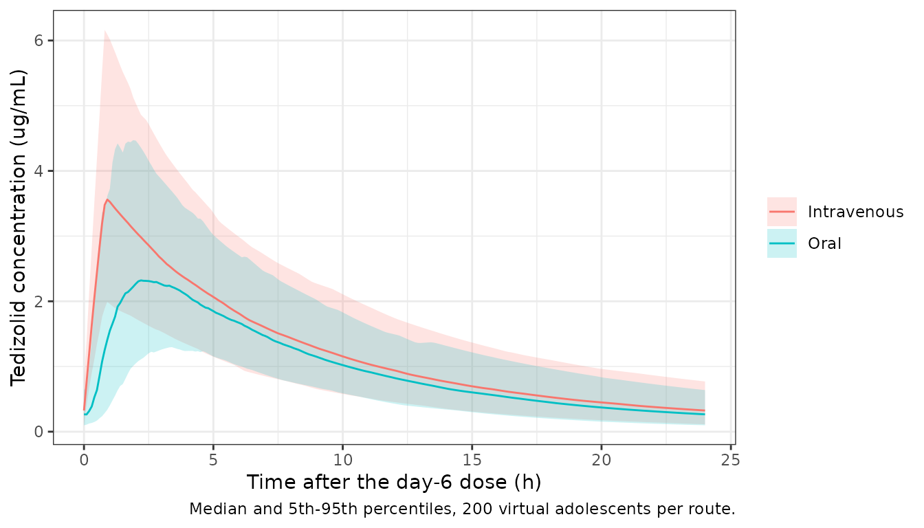
Probability of target attainment (Figure 1)
Figure 1 gives the probability that a 200 mg once-daily adolescent regimen reaches an fAUC/MIC of at least 3. The text reports the intravenous PTA as 100% up to an MIC of 0.5 ug/mL, then 96.2%, 40.3% and 1.0% at 1, 2 and 4 ug/mL. The oral PTA is 99.8%, 90.0%, 24.8% and 0.1% at 0.5, 1, 2 and 4 ug/mL (Results, “Probability of target attainment”). The paper simulated 1,000 adolescents drawn from NHANES. Here the same 200 virtual adolescents are used per route, with the steady-state day-6 AUC(0-24 h).
The Methods give the unbound fraction as 1 - 0.873 = 0.127 (mean protein binding 87.3%), while the Introduction describes tedizolid as about 80% bound. Both are shown.
nca_ado_po <- nca_day1_last(
  sim_ado_po |> dplyr::mutate(admin = "Oral"),
  multi_dose_events(ado_ids, ado_wt, "depot", 1L, rep(0L, n_per_arm)) |>
    dplyr::mutate(admin = "Oral"),
  "admin"
)
nca_ado_ivr <- nca_ado_iv |>
  dplyr::mutate(admin = "Intravenous") |>
  dplyr::select(-wt_band)

auc_ss <- dplyr::bind_rows(nca_ado_ivr, nca_ado_po) |>
  dplyr::filter(PPTESTCD == "auclast", day == "last") |>
  dplyr::select(admin, id, auc = PPORRES)

mics <- c(0.5, 1, 2, 4)
pta <- tidyr::expand_grid(
  auc_ss,
  fu = c(0.127, 0.20),
  mic = mics
) |>
  dplyr::group_by(admin, fu, mic) |>
  dplyr::summarise(pta = 100 * mean(fu * auc / mic >= 3), .groups = "drop")

published_pta <- tibble::tribble(
  ~admin,        ~mic, ~published,
  "Intravenous", 0.5,  100,
  "Intravenous", 1,    96.2,
  "Intravenous", 2,    40.3,
  "Intravenous", 4,    1.0,
  "Oral",        0.5,  99.8,
  "Oral",        1,    90.0,
  "Oral",        2,    24.8,
  "Oral",        4,    0.1
)

pta_wide <- pta |>
  dplyr::mutate(fu = paste0("fu_", fu)) |>
  tidyr::pivot_wider(names_from = fu, values_from = pta) |>
  dplyr::left_join(published_pta, by = c("admin", "mic"))

pta_wide |>
  dplyr::rename(
    "Route" = admin,
    "MIC (ug/mL)" = mic,
    "PTA %, fu 0.127" = fu_0.127,
    "PTA %, fu 0.20" = fu_0.2,
    "PTA %, published" = published
  ) |>
  knitr::kable(
    digits = 1,
    caption = "Replicates the PTA values of Figure 1 of Li 2021 (fAUC/MIC >= 3)."
)| Route | MIC (ug/mL) | PTA %, fu 0.127 | PTA %, fu 0.20 | PTA %, published |
|---|---|---|---|---|
| Intravenous | 0.5 | 99.5 | 100.0 | 100.0 |
| Intravenous | 1.0 | 74.0 | 96.0 | 96.2 |
| Intravenous | 2.0 | 7.5 | 47.5 | 40.3 |
| Intravenous | 4.0 | 0.0 | 2.0 | 1.0 |
| Oral | 0.5 | 99.5 | 99.5 | 99.8 |
| Oral | 1.0 | 50.5 | 94.5 | 90.0 |
| Oral | 2.0 | 2.5 | 25.0 | 24.8 |
| Oral | 4.0 | 0.0 | 0.5 | 0.1 |
ggplot(pta, aes(mic, pta, colour = factor(fu))) +
  geom_line() +
  geom_point() +
  geom_point(
    data = published_pta, aes(mic, published),
    inherit.aes = FALSE, shape = 4, size = 3
  ) +
  facet_wrap(~admin) +
  scale_x_log10(breaks = mics) +
  labs(
    x = "MIC (ug/mL)", y = "PTA (%)", colour = "Unbound fraction",
    caption = "Crosses: PTA values reported in the text of Li 2021."
  ) +
  theme_bw()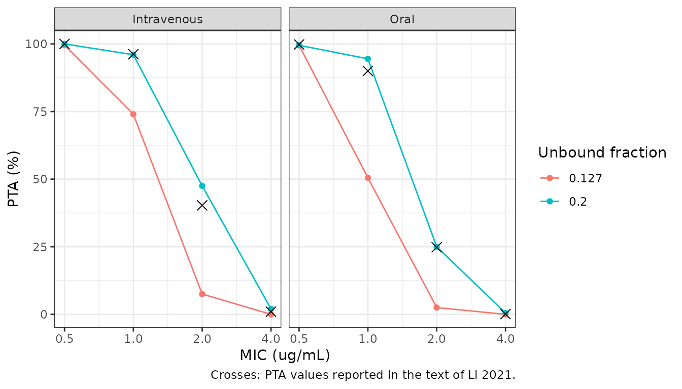
The published curve is reproduced with an unbound fraction of about 0.20 (80% binding) and not with the 0.127 given in the Methods. At 0.127 the PTA at an MIC of 1 ug/mL falls to about 50-75%, far below the published 90-96%. The exposures themselves match Table 3, so the gap lies in the PK/PD step and not in the PK model. Either the figure used the ~80% binding quoted in the Introduction, or the Methods value does not describe the calculation. The conclusion the paper draws, 100% PTA up to the 0.5 ug/mL breakpoint, holds under both values.
pta_check <- pta_wide |> dplyr::filter(mic %in% c(1, 2))
stopifnot(
  # The ~80%-binding curve tracks the published PTA at the two informative
  # MICs, and the 87.3%-binding curve does not.
  stats::median(abs(pta_check$fu_0.2 - pta_check$published)) < 10,
  stats::median(abs(pta_check$fu_0.127 - pta_check$published)) > 20,
  # PTA at the 0.5 ug/mL breakpoint is essentially 100% under either value.
  all(pta_wide$fu_0.2[pta_wide$mic == 0.5] > 97)
)
Assumptions and deviations
- Dose basis. The model is dosed in tedizolid free-base equivalents, so 200 mg tedizolid phosphate is 164.5 mg. The paper does not state the basis. The Table 3 weight-quartile AUCs pick this basis over the prodrug mass, which would overpredict every AUC by about 22%.
-
IIV scale. Table 1 prints IIV as %CV. The variances
use
omega^2 = log(CV^2 + 1), the log-normal relation; for the 258% CV on the zero-order duration this gives 2.036, against 6.66 if the CV were read assqrt(omega^2). The paper does not state which convention it used. -
Residual-error combination. Table 1 gives the
patient-trial and oral-data terms as separate fold-increases of the
residual SD (“on the square root scale”). They are applied
multiplicatively, so an oral record from a patient trial has SD 0.123 *
4.92 * 2.01 = 1.22 on the log scale. The paper does not state whether
the two factors combine or one overrides the other. The residual error
is exponential (
lnorm), following the log error model of the Flanagan 2014 backbone. Residual error does not affect any comparison in this article. -
Study 104 coding. The phase 2 ABSSSI study 104
shares the phase 3 residual-error stratum, so
STUDY_PHASE3 = 1should be set for it. -
Infection covariate. The source flag
INFECis carried asDIS_CSSSI(ABSSSI), because the Results name ABSSSI as the covariate and the reference was changed to healthy volunteers. How the 41 hospitalized pediatric participants with suspected (unconfirmed) infection were coded is not reported. -
Missing diabetes status. Status was missing (-99)
for 232 participants. How that code entered the covariate equation is
not reported. The model takes
DIS_DIABas 0 or 1. - Weight exponents. The Methods say the weight exponents were fixed during the update, but Table 1 prints an RSE for each and does not mark them fixed. They are carried as estimated values.
-
Infusion time. Intravenous doses are infused over
the modelled duration
d2(0.810 h, fixed, with a fixed 8.26% CV IIV) rather than a duration taken from the data set. Dose records must carryrate = -2. -
Bootstrap disagreement. The bootstrap means for the
zero-order duration (0.475 h against 0.175 h),
ka(0.964 against 1.47 1/h) and lag time (0.178 against 0.226 h) differ from the final estimates. Only 432 of 1,000 bootstrap runs were successful, and the bootstrap used FOCE while the final model used SAEM. The final-model values are used. - Virtual cohorts. The PN012 weight distribution is log-normal, fitted to the median and range of supplement Table A2, with all PN012 participants dosed intravenously. The paper’s PTA drew adolescents from NHANES; this article reuses the PN012-like cohort, which Figure A3 shows to have a comparable weight distribution.
- Exposure-response. The paper found no exposure-efficacy or exposure-safety relationship (Figures 2 and 3) and fitted no model, so there is nothing further to encode.