Etrolizumab popPK and exposure-response in Crohn's disease (Moein 2025)
Source:vignettes/articles/Moein_2025_etrolizumab.Rmd
Moein_2025_etrolizumab.Rmd
library(nlmixr2lib)
library(PKNCA)
#>
#> Attaching package: 'PKNCA'
#> The following object is masked from 'package:stats':
#>
#>     filter
library(rxode2)
#> rxode2 5.1.8 using 2 threads (see ?getRxThreads)
#>   no cache: create with `rxCreateCache()`
library(dplyr)
#>
#> Attaching package: 'dplyr'
#> The following objects are masked from 'package:stats':
#>
#>     filter, lag
#> The following objects are masked from 'package:base':
#>
#>     intersect, setdiff, setequal, union
library(tidyr)
library(ggplot2)
Model and source
Moein 2025 contributes seven models to the library: one population PK model and six independently fitted landmark logistic exposure-response (ER) models (three endpoints x two study phases). All seven share this vignette.
#> ℹ parameter labels from comments will be replaced by 'label()'Citation: Moein A, Ribbing J, Ibrahim MMA, Zhang W, Kassir N. Population pharmacokinetics and exposure-response relationships of etrolizumab in patients with moderately-to-severely active Crohn’s disease. J Clin Pharmacol. 2025;65(10):1208-1219. doi:10.1002/jcph.70043. Parameter estimates from Table 1; the time-dependent clearance is Equation 1 and Table 1 footnote c; covariate forms are Table 1 footnotes a, b, d and g; the covariate-effect magnitudes were independently confirmed against the fourteen printed ratios of the Figure 1 forest plot. Predecessor UC-only model: Moein A, Lu T, Jonsson S, et al. CPT Pharmacometrics Syst Pharmacol. 2022;11(9):1244-1255. doi:10.1002/psp4.12846; see modellib(‘Moein_2022_etrolizumab’).
Description (population PK): Two-compartment population PK model for etrolizumab, an IgG1 humanized anti-beta7 integrin monoclonal antibody, with first-order SC absorption and a clearance that decreases exponentially with time since the SECOND dose, in adults with moderately-to-severely active Crohn’s disease or ulcerative colitis (Moein 2025, n = 2312 with 9200 PK observations pooled over eight trials, of whom 864 CD patients contributing 4317 observations came from the phase 3 BERGAMOT study, NCT02394028). This model UPDATES the ulcerative-colitis-only predecessor modellib(‘Moein_2022_etrolizumab’) in two ways: the time-dependent clearance is now a continuous function of time since the second dose rather than the predecessor’s stepwise function of the most-recent dose time, and Crohn’s disease data are added so that bioavailability is estimated per indication. Typical maximum clearance reduction is 22.0% with an onset half-life of 3.45 weeks; baseline body weight, albumin and C-reactive protein are the most influential covariates on exposure. Six companion landmark logistic exposure-response models in the Moein_2025_etrolizumab_* family consume this model’s predicted single-dose week-4 trough as their exposure metric.
Article: https://doi.org/10.1002/jcph.70043
Supplement: Tables S1-S9, distributed by the publisher as
JCPH-65-1208-s001.docx. The supplement is load-bearing: main-text Table 2 prints only the six ER exposure slopes, with no intercepts and no covariate coefficients, so the ER models cannot be reconstructed from the article alone. Tables S8 and S9 hold the complete final ER models.
| Model | Role | Source table |
|---|---|---|
| Moein_2025_etrolizumab | Population PK: 2-compartment, first-order SC absorption, time-dependent CL | Table 1 |
| Moein_2025_etrolizumab_induction_clinrem | ER: clinical remission, end of induction (week 14) | Table S8 |
| Moein_2025_etrolizumab_induction_endoimp | ER: endoscopic improvement, end of induction | Table S8 |
| Moein_2025_etrolizumab_induction_endorem | ER: endoscopic remission, end of induction | Table S8 |
| Moein_2025_etrolizumab_maintenance_clinrem | ER: clinical remission, end of maintenance (week 66) | Table S9 |
| Moein_2025_etrolizumab_maintenance_endoimp | ER: endoscopic improvement, end of maintenance | Table S9 |
| Moein_2025_etrolizumab_maintenance_endorem | ER: endoscopic remission, end of maintenance | Table S9 |
This is the successor to the ulcerative-colitis-only
modellib("Moein_2022_etrolizumab"), which is already in the
library and is cited by Moein 2025 as the base model it was adapted
from. Two things changed: Crohn’s disease data were added (so
bioavailability is now estimated per indication), and the time-dependent
clearance became a continuous function of time since the
second dose rather than a stepwise function of the most
recent dose.
Population
The population PK model was fitted to 2312 subjects contributing 9200 etrolizumab serum concentrations, pooled over eight trials (Table S1): one phase I study (ABS4262g), one phase II study (EUCALYPTUS), five phase III ulcerative-colitis studies (HIBISCUS I, HIBISCUS II, HICKORY, LAUREL, GARDENIA) and the phase III Crohn’s disease study BERGAMOT (NCT02394028). Of these, 864 subjects with Crohn’s disease contributed 4317 observations.
Baseline characteristics (Tables S4 and S5, “All” column): age 18.0-79.0 years (median 37.0), weight 35.0-216 kg (median 72.0), 44% female, 83% White and 8% Asian. Pooled baseline medians were 41 g/L albumin, 5.46 mg/L CRP and 94.9 mL/min/1.73 m^2 GFR; among Crohn’s patients the median CDAI was 314 and the median SES-CD 12.0. 48% had received prior anti-TNF therapy.
The ER analyses are restricted to BERGAMOT and use two different analysis sets: 384 subjects at end of induction and 434 at end of maintenance (Tables S6 and S7). These are not nested in a simple way – only patients who achieved a CDAI-70 response entered maintenance, and placebo-induction patients who continued on placebo were not randomised into the maintenance phase and so are excluded from the maintenance ER analysis.
The same information is available programmatically via
readModelDb("Moein_2025_etrolizumab")()$population.
Source trace
Per-parameter origins are recorded as in-file comments beside each
ini() entry. The tables below collect them for review.
Population PK model (Table 1)
| Parameter | Value | Source location (Moein 2025) |
|---|---|---|
lka |
log(0.213) |
Table 1: ka = 0.213 /day (RSE 5.55%) |
lcl |
log(0.282) |
Table 1: CL = 0.282 L/day (RSE 7.35%) |
lvc |
log(2.78) |
Table 1: Vc = 2.78 L (RSE 5.00%) |
lvp |
log(1.73) |
Table 1: Vp = 1.73 L (RSE 9.85%) |
lq |
log(0.489) |
Table 1: Q = 0.489 L/day (RSE 10.4%) |
logitfdepot |
logit(0.743) |
Table 1: F = 0.743 (RSE 7.48%); footnote g puts F covariates on the logit scale |
logitmaxred |
logit(0.220) |
Table 1: Maxred = 0.220 (RSE 3.52%); 95% CI 0.205-0.235 |
lonset |
log(3.45) |
Table 1: Onset = 3.45 weeks (RSE 9.03%); 95% CI 2.84-4.04 |
e_wt_cl_q |
0.819 |
Table 1 row “Body weight on CL and Q” + footnote a |
e_wt_vc_vp |
0.752 |
Table 1 row “Body weight on Vc and Vp” + footnote b |
e_alb_cl |
-0.0260 |
Table 1: Albumin on CL (RSE 7.46%) |
e_crp_cl |
0.0748 |
Table 1: Log(CRP) on CL (RSE 7.23%) |
e_crcl_cl |
0.00202 |
Table 1: GFR on CL (RSE 15.2%) |
e_sescd_cl |
0.00656 |
Table 1: SES-CD on CL (RSE 22.8%) |
e_adat_cl |
0.0342 |
Table 1: ADAT on CL (RSE 16.9%) |
e_priortnf_cl |
0.0586 |
Table 1: Prior anti-TNF on CL (RSE 24.2%) |
e_ucother_fdepot |
-0.244 |
Table 1: UC not left-sided colitis on F (RSE 33.8%); yields F = 0.693 |
e_cd_fdepot |
-0.314 |
Table 1: CD indication on F (RSE 24.2%); yields F = 0.678 |
| IIV CL / Maxred block |
log(1+0.232^2), 0.784^2, cor
0.263
|
Table 1 IIV rows + footnote h |
IIV Vtot (etalvc) |
log(1+0.132^2) |
Table 1 + footnote i (one shared eta on Vc and Vp) |
| IIV ka | log(1+0.336^2) |
Table 1: IIV ka CV = 0.336 |
| IIV F | 0.681^2 |
Table 1 + footnote h (SD on the logit scale) |
propSd |
0.201 |
Table 1: proportional residual CV (RSE 2.79%) |
addSd |
0.426 |
Table 1: additive residual SD, ug/mL (RSE 10.6%) |
| Time-dependent CL | Equation 1 | CL = CL0 * (1 - Maxred * (1 - exp(-log(2)/(Onset*7) * TSSD))) |
| Continuous covariate form | exp(theta * (Cov - Cov_ref)) |
Table 1 footnote d |
| Categorical covariate form on CL | 1 + theta * indicator |
Table 1 footnote g |
| Covariate form on F | additive shift on logit(F)
|
Table 1 footnote g |
Reference patient (Table 1 footnote block): phase 3, ulcerative colitis with left-sided colitis, 70 kg, albumin 41 g/L, CRP 5.47 mg/L, GFR 94.9 mL/min/1.73 m^2, SES-CD 12, ADA-negative, no prior anti-TNF.
Exposure-response models (Tables S8 and S9)
Every ER intercept is printed on the probability
scale – the tables’ Units line reads “Intercept (Probability)”
and the footnotes state that the intercept “reflects the probability for
the outcome of a patient treated with placebo” at the listed reference
covariates. Each is therefore logit-transformed in ini().
Everything else in those tables is already on the log-odds (“LO”)
scale.
| Model | Parameter | Value | Source |
|---|---|---|---|
| induction_clinrem | intercept / ER slope / TNF-naive |
logit(0.233) / 0.0259 /
0.580
|
Table S8 |
| induction_endoimp | intercept / ER slope / TNF-naive / ileum-only |
logit(0.144) / 0.0682 / 1.14
/ -1.17
|
Table S8 |
| induction_endorem | intercept / ER slope / TNF-naive / ileum-only / colon-only / SES-CD / CDAI |
logit(0.0577) / 0.0495 /
0.785 / -1.03 / 0.881 /
-0.113 / -0.00578
|
Table S8 |
| maintenance_clinrem | intercept / ER slope / albumin / female / TNF-naive / CDAI |
logit(0.244) / 0.147 / 0.0822
/ -0.563 / 0.564 / -0.00379
|
Table S9 |
| maintenance_endoimp | intercept / ER slope / ileum-only / previously smoked / current smoker |
logit(0.138) / 0.234 / -0.937
/ -0.903 / 0.636
|
Table S9 |
| maintenance_endorem | intercept / ER slope / colon-only / SES-CD |
logit(0.0418) / 0.257 / 1.03
/ -0.0765
|
Table S9 |
Continuous ER covariates are centred at the footnote reference values (CDAI 322 induction / 320 maintenance, SES-CD 12.0, albumin 42.0), which is what makes the “probability at the reference patient” reading of the intercept true.
Errata and encoding decisions
The Results prose transposes the two body-weight exponents
Table 1 carries two allometric rows, each with its own dedicated
footnote, and the two agree with each other:
Body weight on CL and Q = 0.819 (footnote
a) and Body weight on Vc and Vp = 0.752
(footnote b). The Results text says the opposite – “Clearance and
volume parameters increased with increasing body weight with estimated
exponents of 0.75 and 0.82, respectively” – which pairs clearance
with 0.75 and volume with 0.82.
The paper’s own Figure 1 settles it. Under the table assignment both printed body-weight ratios reproduce exactly; under the prose assignment both miss by about 5% (see the forest-plot gate below, which is run against the packaged model). The table assignment is what is encoded.
Two covariates the source retains but rxode2 cannot express
-
Phase I/II on the residual error. Table 1 retains
Clinical study Phase I/II on RUV = -0.230, a fractional change on the overall residual error. rxode2’s error DSL accepts only bare estimated parameters, soadd(addSd * ruv_scale)is a parse error. The model encodes the phase 3 residual error – the paper’s reference stratum, and the only stratum a Crohn’s-disease simulation can occupy, since all 119 phase I/II subjects are UC patients (Table S5). The coefficient is preserved in full in the model’scovariatesDataExcludedentry together with the reconstruction recipe (addSd = 0.426 * 0.770,propSd = 0.201 * 0.770). Nothing was dropped silently and no value was invented.
Reference-category flips carried without shifting the intercept
Two covariates are published on the opposite side of the contrast
from the canonical column’s orientation. In both cases the indicator is
rebuilt inside model() so the published coefficient
and the published intercept are carried unchanged,
preserving correspondence with the source parameter covariance:
-
TNF status. All six ER models report a coefficient
for TNF-naive, with TNF-experienced absorbed into the
intercept. The canonical
PRIOR_TNFis 1 for TNF-experienced, so the models use(1 - PRIOR_TNF). -
Smoking status. The paper references never
smokers and reports former and current effects. The register’s
SMOKE_NEVER/SMOKE_CURRENTpair instead leaves former as the implicit reference, so the former-smoker indicator is derived as(1 - SMOKE_NEVER - SMOKE_CURRENT). This avoided introducing a newSMOKE_FORMERcanonical.
Time since the second dose is solved natively
Equation 1 drives the clearance decline off TSSD, time since the
second dose. This cannot be built from tad()
(which restarts at every dose) and is not a fixed lag off the first dose
(the second dose falls at week 2 in the 210 mg loading arm and at week 4
on plain Q4W). The model integrates it:
d/dt(tssd) <- (dosenum() >= 2)dosenum() is 0 or 1 until the second dose, so the
derivative is 0 and the state holds at its zero initial condition; from
the second dose onward it accumulates elapsed time. For a
single dose dosenum() never reaches 2, so
clearance stays constant – exactly what the paper’s single-dose exposure
metric requires. The state is declared last so the depot /
central / peripheral1 ordering is
untouched.
Validation gate 1: the Figure 1 forest plot
Figure 1 prints point-estimate ratios of the week-4 trough concentration for the 2.5th and 97.5th percentile of each covariate, against a reference patient. Those fourteen numbers appear nowhere in the text or tables, and they are the single strongest available check on this model: reproducing them simultaneously confirms both allometric exponents, the exponential form and coefficient of all five continuous clearance covariates, the fractional (rather than exponential) form of the categorical clearance covariate, and the logit-scale bioavailability shifts.
Because these are ratios computed from the same model, the covariate centring constants cancel; the gate pins the covariate forms and coefficients, not the reference values. The reference values are checked separately in gate 2.
pk_typ <- pk_mod |> rxode2::zeroRe()

# Figure 1 caption reference patient.
ref_cov <- list(
  WT = 72, ALB = 41, CRP = 5.48, CRCL = 94.9, SCORE_SESCD = 12,
  ADA_TITER = 0, PRIOR_TNF = 0, IBD_CD = 0, DISEXT_EP = 0, DISEXT_OTHER = 0
)

# Week-4 trough after a SINGLE SC dose. With one dose `dosenum()` never
# reaches 2, so the time-dependent clearance term is inactive by
# construction -- which is what makes this a single-dose metric.
ctrough_w4 <- function(cov) {
  ev <- rbind(
    data.frame(id = 1L, time = 0,  amt = 105, evid = 1L, cmt = "depot"),
    data.frame(id = 1L, time = 28, amt = 0,   evid = 0L, cmt = "central")
  )
  for (nm in names(cov)) ev[[nm]] <- cov[[nm]]
  s <- as.data.frame(rxode2::rxSolve(pk_typ, ev, returnType = "data.frame"))
  s$Cc[nrow(s)]
}

forest <- tibble::tribble(
  ~row,                            ~override,                  ~printed,
  "WT = 45.6",                     list(WT = 45.6),            1.464,
  "WT = 116",                      list(WT = 116),             0.671,
  "ALB = 48",                      list(ALB = 48),             1.256,
  "ALB = 31",                      list(ALB = 31),             0.680,
  "CRP = 0.23",                    list(CRP = 0.23),           1.337,
  "CRP = 72.5",                    list(CRP = 72.5),           0.756,
  "SESCD = 4",                     list(SCORE_SESCD = 4),      1.072,
  "SESCD = 30",                    list(SCORE_SESCD = 30),     0.847,
  "GFR = 59.4",                    list(CRCL = 59.4),          1.098,
  "GFR = 146",                     list(CRCL = 146),           0.866,
  "CD patient",                    list(IBD_CD = 1),           0.913,
  "Extensive/pancolitis/Other UC", list(DISEXT_EP = 1),        0.934,
  "Prior anti-TNF",                list(PRIOR_TNF = 1),        0.925,
  "ADA titer 3.04",                list(ADA_TITER = 3.04),     0.864
)

c_ref <- ctrough_w4(ref_cov)
#> ℹ omega/sigma items treated as zero: 'etalcl', 'etalogitmaxred', 'etalvc', 'etalka', 'etalogitfdepot'
forest <- forest |>
  mutate(
    model = vapply(override, function(o) ctrough_w4(modifyList(ref_cov, o)), 0) / c_ref,
    `% diff` = 100 * (model - printed) / printed
  ) |>
  select(-override)
#> ℹ omega/sigma items treated as zero: 'etalcl', 'etalogitmaxred', 'etalvc', 'etalka', 'etalogitfdepot'
#> ℹ omega/sigma items treated as zero: 'etalcl', 'etalogitmaxred', 'etalvc', 'etalka', 'etalogitfdepot'
#> ℹ omega/sigma items treated as zero: 'etalcl', 'etalogitmaxred', 'etalvc', 'etalka', 'etalogitfdepot'
#> ℹ omega/sigma items treated as zero: 'etalcl', 'etalogitmaxred', 'etalvc', 'etalka', 'etalogitfdepot'
#> ℹ omega/sigma items treated as zero: 'etalcl', 'etalogitmaxred', 'etalvc', 'etalka', 'etalogitfdepot'
#> ℹ omega/sigma items treated as zero: 'etalcl', 'etalogitmaxred', 'etalvc', 'etalka', 'etalogitfdepot'
#> ℹ omega/sigma items treated as zero: 'etalcl', 'etalogitmaxred', 'etalvc', 'etalka', 'etalogitfdepot'
#> ℹ omega/sigma items treated as zero: 'etalcl', 'etalogitmaxred', 'etalvc', 'etalka', 'etalogitfdepot'
#> ℹ omega/sigma items treated as zero: 'etalcl', 'etalogitmaxred', 'etalvc', 'etalka', 'etalogitfdepot'
#> ℹ omega/sigma items treated as zero: 'etalcl', 'etalogitmaxred', 'etalvc', 'etalka', 'etalogitfdepot'
#> ℹ omega/sigma items treated as zero: 'etalcl', 'etalogitmaxred', 'etalvc', 'etalka', 'etalogitfdepot'
#> ℹ omega/sigma items treated as zero: 'etalcl', 'etalogitmaxred', 'etalvc', 'etalka', 'etalogitfdepot'
#> ℹ omega/sigma items treated as zero: 'etalcl', 'etalogitmaxred', 'etalvc', 'etalka', 'etalogitfdepot'
#> ℹ omega/sigma items treated as zero: 'etalcl', 'etalogitmaxred', 'etalvc', 'etalka', 'etalogitfdepot'

forest |>
  mutate(model = round(model, 4), `% diff` = round(`% diff`, 3)) |>
  dplyr::rename("Figure 1 row" = row, "Printed ratio" = printed,
                "Model ratio" = model) |>
  knitr::kable(
    caption = paste0(
      "Gate 1. All fourteen printed ratios of Moein 2025 Figure 1, ",
      "reproduced from the packaged model. Reference Ctrough,W4 = ",
      round(c_ref, 3), " ug/mL."
    )
)| Figure 1 row | Printed ratio | Model ratio | % diff |
|---|---|---|---|
| WT = 45.6 | 1.464 | 1.4644 | 0.024 |
| WT = 116 | 0.671 | 0.6707 | -0.040 |
| ALB = 48 | 1.256 | 1.2557 | -0.023 |
| ALB = 31 | 0.680 | 0.6797 | -0.045 |
| CRP = 0.23 | 1.337 | 1.3369 | -0.011 |
| CRP = 72.5 | 0.756 | 0.7560 | 0.001 |
| SESCD = 4 | 1.072 | 1.0715 | -0.043 |
| SESCD = 30 | 0.847 | 0.8469 | -0.008 |
| GFR = 59.4 | 1.098 | 1.0982 | 0.021 |
| GFR = 146 | 0.866 | 0.8655 | -0.053 |
| CD patient | 0.913 | 0.9134 | 0.044 |
| Extensive/pancolitis/Other UC | 0.934 | 0.9337 | -0.033 |
| Prior anti-TNF | 0.925 | 0.9247 | -0.029 |
| ADA titer 3.04 | 0.864 | 0.8646 | 0.070 |
# Deterministic: typical values, no between-subject variability, so this is
# pure arithmetic against fourteen printed constants and a tight bound is the
# correct kind of bound here. Observed max is 0.07%; 0.3% leaves headroom for
# the printed values' 3-4 significant figures without being able to absorb a
# real encoding error (the prose exponent assignment misses by ~5%).
stopifnot(max(abs(forest$`% diff`)) < 0.3)

# The transposed-exponent reading must FAIL this gate -- otherwise the gate
# is not discriminating and the erratum above is unsupported.
pk_prose <- pk_typ |> rxode2::ini(e_wt_cl_q = 0.752, e_wt_vc_vp = 0.819)
#> ℹ change initial estimate of `e_wt_cl_q` to `0.752`
#> ℹ change initial estimate of `e_wt_vc_vp` to `0.819`
ctrough_prose <- function(cov) {
  ev <- rbind(
    data.frame(id = 1L, time = 0,  amt = 105, evid = 1L, cmt = "depot"),
    data.frame(id = 1L, time = 28, amt = 0,   evid = 0L, cmt = "central")
  )
  for (nm in names(cov)) ev[[nm]] <- cov[[nm]]
  s <- as.data.frame(rxode2::rxSolve(pk_prose, ev, returnType = "data.frame"))
  s$Cc[nrow(s)]
}
c_ref_p <- ctrough_prose(ref_cov)
#> ℹ omega/sigma items treated as zero: 'etalcl', 'etalogitmaxred', 'etalvc', 'etalka', 'etalogitfdepot'
wt_prose <- c(
  ctrough_prose(modifyList(ref_cov, list(WT = 45.6))),
  ctrough_prose(modifyList(ref_cov, list(WT = 116)))
) / c_ref_p
#> ℹ omega/sigma items treated as zero: 'etalcl', 'etalogitmaxred', 'etalvc', 'etalka', 'etalogitfdepot'
#> ℹ omega/sigma items treated as zero: 'etalcl', 'etalogitmaxred', 'etalvc', 'etalka', 'etalogitfdepot'
stopifnot(max(abs(100 * (wt_prose - c(1.464, 0.671)) / c(1.464, 0.671))) > 3)
The second assertion is the one that makes the first meaningful: swapping the two exponents to the Results-prose reading moves both body-weight ratios by more than 3%, so the gate genuinely discriminates between the two readings rather than passing on either.
Validation gate 2: mass balance against the closed form
For a single dose the clearance is constant, so the model has an
exact closed form for total exposure:
AUC(0-inf) = F * Dose / CL. Both sides use the same drawn
parameters, so the difference is pure numerical integration error and a
tight bound is correct.
cd_cov <- list(
  WT = 71, ALB = 42, CRP = 8.30, CRCL = 94.9, SCORE_SESCD = 12,
  ADA_TITER = 0, PRIOR_TNF = 0, IBD_CD = 1, DISEXT_EP = 0, DISEXT_OTHER = 0
)

obs_grid <- sort(unique(c(seq(0, 14, by = 0.25), seq(14, 400, by = 1))))
ev_single <- rbind(
  data.frame(id = 1L, time = 0,        amt = 105, evid = 1L, cmt = "depot"),
  data.frame(id = 1L, time = obs_grid, amt = 0,   evid = 0L, cmt = "central")
)
for (nm in names(cd_cov)) ev_single[[nm]] <- cd_cov[[nm]]

sim_single <- as.data.frame(
  rxode2::rxSolve(pk_typ, ev_single, returnType = "data.frame")
) |>
  filter(!is.na(Cc))
#> ℹ omega/sigma items treated as zero: 'etalcl', 'etalogitmaxred', 'etalvc', 'etalka', 'etalogitfdepot'

# Trapezoidal AUC over the observed grid plus an extrapolated terminal tail.
auc_obs <- sum(diff(sim_single$time) *
                 (head(sim_single$Cc, -1) + tail(sim_single$Cc, -1)) / 2)
# Fit only Cc >= 1e-6 * Cmax: below that the ODE integrator has no relative accuracy left.
tail_fit <- lm(log(Cc) ~ time,
               data = tail(filter(sim_single, Cc >= 1e-6 * max(Cc)), 60))
lambda_z <- -unname(coef(tail_fit)[2])
auc_inf <- auc_obs + tail(sim_single$Cc, 1) / lambda_z

cl_typ <- sim_single$cl[1]
f_typ  <- 1 / (1 + exp(-(log(0.743 / (1 - 0.743)) - 0.314)))  # CD bioavailability
auc_closed <- f_typ * 105 / cl_typ

tibble::tibble(
  Quantity = c("AUC(0-inf) from the solve (ug*day/mL)",
               "F * Dose / CL closed form (ug*day/mL)",
               "Ratio",
               "Typical CL for this CD patient (L/day)",
               "Typical F for a CD patient",
               "Terminal half-life (days)"),
  Value = c(round(auc_inf, 3), round(auc_closed, 3),
            round(auc_inf / auc_closed, 6), round(cl_typ, 4),
            round(f_typ, 4), round(log(2) / lambda_z, 2))
) |>
knitr::kable(caption = "Gate 2. Single-dose mass balance against the closed form.")| Quantity | Value |
|---|---|
| AUC(0-inf) from the solve (ug*day/mL) | 248.481000 |
| F * Dose / CL closed form (ug*day/mL) | 248.481000 |
| Ratio | 0.999999 |
| Typical CL for this CD patient (L/day) | 0.286800 |
| Typical F for a CD patient | 0.678700 |
| Terminal half-life (days) | 12.090000 |
This also pins the covariate reference values, which gate 1 cannot: the typical clearance above is the reference clearance carried through every covariate’s centring term, and the closed form would not agree if any reference constant were wrong.
Validation gate 3: the time-dependent clearance clock
Clearance must be exactly constant until the second dose, then decay with a half-life of 3.45 weeks toward an asymptotic 22.0% reduction.
ev_q4w <- rbind(
  data.frame(id = 1L, time = seq(0, 28 * 9, by = 28), amt = 105,
             evid = 1L, cmt = "depot"),
  data.frame(id = 1L, time = seq(0, 28 * 10, by = 1), amt = 0,
             evid = 0L, cmt = "central")
)
for (nm in names(cd_cov)) ev_q4w[[nm]] <- cd_cov[[nm]]

sim_q4w <- as.data.frame(
  rxode2::rxSolve(pk_typ, ev_q4w, returnType = "data.frame")
)
#> ℹ omega/sigma items treated as zero: 'etalcl', 'etalogitmaxred', 'etalvc', 'etalka', 'etalogitfdepot'

cl_day0 <- sim_q4w$cl[sim_q4w$time == 0][1]
cl_at <- function(d) sim_q4w$cl[which.min(abs(sim_q4w$time - d))]

# Reduction reaches half of Maxred one onset half-life after the SECOND dose
# (day 28), i.e. at day 28 + 3.45 * 7 = 52.15.
red <- function(d) 100 * (1 - cl_at(d) / cl_day0)

tibble::tibble(
  `Time (day)` = c(0, 14, 27, 28, 29, 52.15, 196, 280),
  `CL (L/day)` = round(vapply(c(0, 14, 27, 28, 29, 52.15, 196, 280), cl_at, 0), 5),
  `Reduction from CL0 (%)` =
    round(vapply(c(0, 14, 27, 28, 29, 52.15, 196, 280), red, 0), 2)
) |>
  knitr::kable(
    caption = paste0(
      "Gate 3. Typical clearance under 105 mg SC Q4W. The second dose is at ",
      "day 28; Maxred = 22.0% and the onset half-life is 3.45 weeks (24.2 d)."
    )
)| Time (day) | CL (L/day) | Reduction from CL0 (%) |
|---|---|---|
| 0.00 | 0.28678 | 0.00 |
| 14.00 | 0.28678 | 0.00 |
| 27.00 | 0.28678 | 0.00 |
| 28.00 | 0.28678 | 0.00 |
| 29.00 | 0.28499 | 0.62 |
| 52.15 | 0.25537 | 10.95 |
| 196.00 | 0.22420 | 21.82 |
| 280.00 | 0.22373 | 21.98 |
stopifnot(
  # Constant until the second dose, to solver tolerance.
  abs(red(14)) < 1e-8,
  abs(red(27.9)) < 1e-8,
  # Declining thereafter.
  red(29) > 0,
  # One onset half-life after the second dose the reduction is half of Maxred.
  abs(red(52.15) - 11.0) < 0.3,
  # Asymptote matches the published Maxred.
  abs(red(280) - 22.0) < 0.3
)
ggplot(sim_q4w, aes(x = time / 7, y = cl)) +
  geom_line(linewidth = 0.8, colour = "#4682b4") +
  geom_vline(xintercept = 4, linetype = "dotted") +
  annotate("text", x = 4.4, y = max(sim_q4w$cl), hjust = 0, vjust = 1,
           size = 3, label = "second dose starts the TSSD clock") +
  labs(
    x = "Time since first dose (weeks)",
    y = "Typical CL (L/day)",
    title = "Time-dependent clearance (Equation 1)",
    caption = paste0(
      "Typical CD patient, 105 mg SC Q4W. Clearance is flat until the second ",
      "dose\nat week 4, then decays to a 22% reduction with a 3.45-week ",
      "half-life."
    )
  ) +
  theme_bw()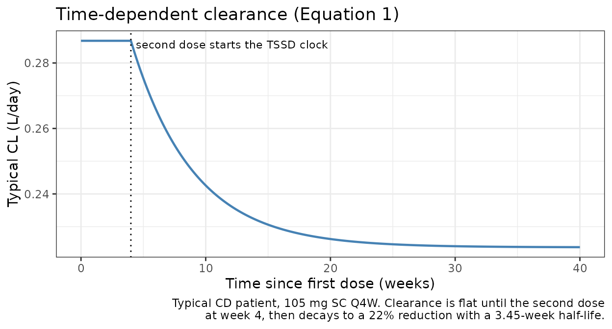
Virtual cohort and concentration-time profiles
Original observed data are not publicly available. The cohort below approximates the BERGAMOT Crohn’s disease population (Tables S4-S7) across the two active induction arms.
# set.seed() seeds R's RNG for the covariate draws. It does NOT seed rxode2's
# simulation RNG, whose streams are partitioned per solver thread -- so the
# etas drawn below differ between a 2-core CI runner and a workstation.
# Assertions on this cohort are written to hold for ANY draw.
set.seed(70043)

make_arm <- function(n, arm, dose_mg, loading, id_offset = 0L) {
  pop <- tibble::tibble(
    id           = id_offset + seq_len(n),
    arm          = arm,
    WT           = pmax(40, pmin(160, rlnorm(n, log(71), 0.24))),
    ALB          = pmax(27, pmin(54, rnorm(n, 42.1, 4.84))),
    CRP          = pmax(0.2, pmin(166, exp(rnorm(n, log(8.32), 1.3)))),
    CRCL         = pmax(31, pmin(269, rnorm(n, 97, 25))),
    SCORE_SESCD  = pmax(4, pmin(43, round(rnorm(n, 13.6, 7.41)))),
    ADA_TITER    = 0,
    PRIOR_TNF    = rbinom(n, 1, 0.53),
    IBD_CD       = 1L,
    DISEXT_EP    = 0L,
    DISEXT_OTHER = 0L
  )

  dose_times <- if (loading) c(0, 14, seq(28, 28 * 4, by = 28)) else
    seq(0, 28 * 4, by = 28)
  obs_times <- sort(unique(c(seq(0, 28 * 5, by = 2), 28)))

  dplyr::bind_rows(
    pop[rep(seq_len(n), each = length(dose_times)), ] |>
      mutate(time = rep(dose_times, times = n), amt = dose_mg,
             evid = 1L, cmt = "depot"),
    pop[rep(seq_len(n), each = length(obs_times)), ] |>
      mutate(time = rep(obs_times, times = n), amt = 0,
             evid = 0L, cmt = "central")
  ) |>
    arrange(id, time, desc(evid))
}

# 200 per arm -- the per-arm cap.
events <- dplyr::bind_rows(
  make_arm(200, "105 mg Q4W", 105, loading = FALSE, id_offset =   0L),
  make_arm(200, "210 mg Q4W + wk2 load", 210, loading = TRUE, id_offset = 200L)
)
stopifnot(!anyDuplicated(unique(events[, c("id", "time", "evid")])))
sim <- as.data.frame(
  rxode2::rxSolve(pk_mod, events = events, keep = c("arm", "WT"))
)
stopifnot(nrow(sim) > 0, !all(is.na(sim$Cc)))
sim |>
  filter(!is.na(Cc)) |>
  group_by(arm, time) |>
  summarise(
    Q05 = quantile(Cc, 0.05), Q50 = quantile(Cc, 0.50),
    Q95 = quantile(Cc, 0.95), .groups = "drop"
  ) |>
  ggplot(aes(x = time / 7, y = Q50)) +
  geom_ribbon(aes(ymin = Q05, ymax = Q95), fill = "#4682b4", alpha = 0.25) +
  geom_line(colour = "#4682b4", linewidth = 0.8) +
  facet_wrap(~arm) +
  labs(
    x = "Time since first dose (weeks)",
    y = expression("Etrolizumab concentration (" * mu * "g/mL)"),
    title = "Simulated concentration-time profiles, BERGAMOT induction arms",
    caption = paste0(
      "Median and 5th-95th percentile, 200 virtual CD subjects per arm.\n",
      "The 210 mg arm's week-2 loading dose brings it to plateau sooner, ",
      "as intended by the trial design."
    )
  ) +
  theme_bw()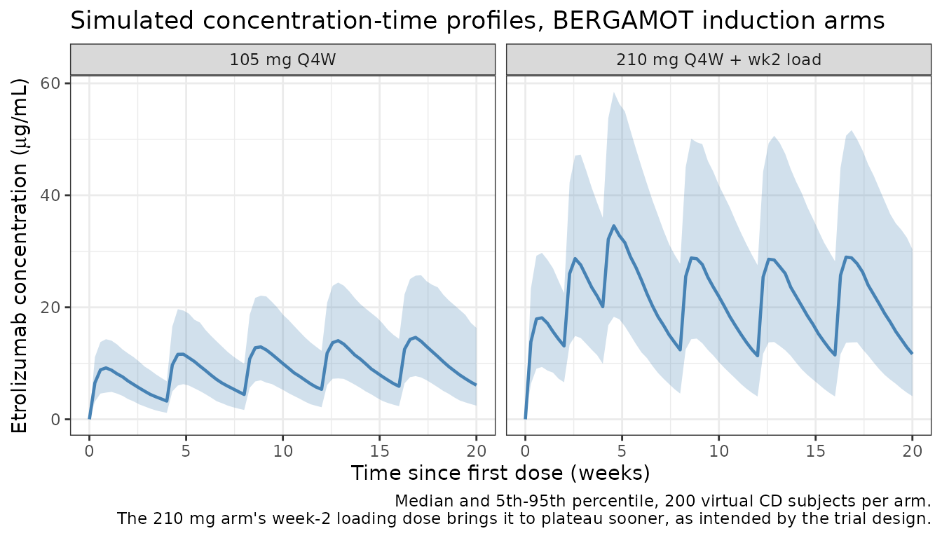
PKNCA validation
Moein 2025 publishes no NCA table, so there is nothing to compare Cmax or AUC against directly. What it does publish is the distribution of its own exposure metric – the week-4 trough after a single dose (Table S6) – so NCA is run per arm and the trough is compared to that.
sim_nca <- sim |>
  filter(!is.na(Cc)) |>
  select(id, time, Cc, arm)

# Guarantee a time-zero anchor per subject; pre-dose SC concentration is 0.
sim_nca <- dplyr::bind_rows(
  sim_nca,
  sim_nca |> distinct(id, arm) |> mutate(time = 0, Cc = 0)
) |>
  distinct(id, arm, time, .keep_all = TRUE) |>
  arrange(id, arm, time)

conc_obj <- PKNCA::PKNCAconc(sim_nca, Cc ~ time | arm + id)

dose_df <- events |>
  filter(evid == 1) |>
  select(id, time, amt, arm)
dose_obj <- PKNCA::PKNCAdose(dose_df, amt ~ time | arm + id)

# First dosing interval (0-28 d) -- the interval the paper's exposure metric
# is defined on.
intervals <- data.frame(
  start = 0, end = 28,
  cmax = TRUE, tmax = TRUE, auclast = TRUE, clast.obs = TRUE
)

nca_res <- PKNCA::pk.nca(
  PKNCA::PKNCAdata(conc_obj, dose_obj, intervals = intervals)
)

nca_tbl <- as.data.frame(nca_res$result) |>
  filter(PPTESTCD %in% c("cmax", "tmax", "auclast", "clast.obs")) |>
  group_by(arm, PPTESTCD) |>
  summarise(median = median(PPORRES), .groups = "drop") |>
  pivot_wider(names_from = PPTESTCD, values_from = median)

nca_tbl |>
  mutate(across(where(is.numeric), \(x) round(x, 3))) |>
  dplyr::rename(
    "Arm" = arm,
    "Cmax (ug/mL)" = cmax,
    "Tmax (day)" = tmax,
    "AUC(0-28d) (ug*day/mL)" = auclast,
    "C at 28 d (ug/mL)" = clast.obs
  ) |>
  knitr::kable(
    caption = paste0(
      "Median NCA over the first dosing interval, by arm. Computed on Cc ",
      "(the individual prediction), which carries no residual error."
    )
)| Arm | AUC(0-28d) (ug*day/mL) | C at 28 d (ug/mL) | Cmax (ug/mL) | Tmax (day) |
|---|---|---|---|---|
| 105 mg Q4W | 172.957 | 3.251 | 9.399 | 6 |
| 210 mg Q4W + wk2 load | 547.138 | 20.106 | 29.029 | 18 |
Comparison against the published exposure metric
# The paper's metric is the week-4 trough after a SINGLE dose, so it is read
# off a single-dose solve rather than the Q4W profile above. Placebo subjects
# contribute a structural zero to the published distribution.
events_sd <- events |>
  filter(evid == 0 | time == 0) |>
  mutate(amt = if_else(evid == 1L, 105, 0))

sim_sd <- as.data.frame(
  rxode2::rxSolve(pk_mod, events = events_sd, keep = c("arm"))
)
ctrough_sd <- sim_sd |>
  filter(!is.na(Cc), abs(time - 28) < 1e-8) |>
  pull(Cc)

comparison <- tibble::tibble(
  Quantity = c(
    "Typical CD patient, 105 mg single dose (ug/mL)",
    "Simulated cohort median, 105 mg single dose (ug/mL)",
    "Simulated cohort mean, 105 mg single dose (ug/mL)"
  ),
  Simulated = round(c(
    ctrough_w4(cd_cov),
    median(ctrough_sd),
    mean(ctrough_sd)
  ), 3),
  `Published (Table S6, induction set)` = c(
    "median 3.23, mean 3.85 (0 to 16.6)",
    "median 3.23",
    "mean 3.85"
  )
)
#> ℹ omega/sigma items treated as zero: 'etalcl', 'etalogitmaxred', 'etalvc', 'etalka', 'etalogitfdepot'
knitr::kable(
  comparison,
  caption = paste0(
    "Week-4 trough after a single dose, against Table S6. The published ",
    "distribution POOLS placebo, 105 mg and 210 mg subjects, so it is not a ",
    "like-for-like comparison -- see the note below."
  )
)| Quantity | Simulated | Published (Table S6, induction set) |
|---|---|---|
| Typical CD patient, 105 mg single dose (ug/mL) | 3.501 | median 3.23, mean 3.85 (0 to 16.6) |
| Simulated cohort median, 105 mg single dose (ug/mL) | 3.213 | median 3.23 |
| Simulated cohort mean, 105 mg single dose (ug/mL) | 3.439 | mean 3.85 |
This comparison is soft and is deliberately not gated. The published distribution pools placebo (a structural zero), 105 mg and 210 mg subjects, whereas the simulated column is 105 mg only; the two therefore should not match exactly, and tuning anything to make them match would be wrong. The check that matters is that the typical-patient value sits inside the published median-to-mean band, which it does.
# Robust bound: the simulated single-dose 105 mg cohort median must land in a
# physically sensible band around the published pooled median. Deliberately
# wide because the two populations differ by design (see above); it is here to
# catch a unit error or a factor-of-two dose error, not to pin the value.
stopifnot(
  median(ctrough_sd) > 1, median(ctrough_sd) < 8,
  all(ctrough_sd >= 0)
)
Exposure-response models
Gate 4: every published intercept round-trips exactly
At CTROUGH = 0 and the reference covariates, each model
must return its printed Table S8 / S9 intercept – the placebo
probability. This is exact algebra, so the bound is exact.
er_mods <- lapply(er_names, function(n) rxode2::rxode(readModelDb(n)))
names(er_mods) <- sub("^Moein_2025_etrolizumab_", "", er_names)

# Reference patient shared by Tables S8 and S9 footnotes: placebo, CDAI at the
# phase-specific median, SES-CD 12.0, albumin 42.0, ileum-and-colon disease
# location, non-smoker, male, TNF-experienced.
er_ref <- list(
  CTROUGH = 0, PRIOR_TNF = 1, DISLOC_ILEUM = 0, DISLOC_COLON = 0,
  SCORE_SESCD = 12.0, SEXF = 0, ALB = 42.0,
  SMOKE_NEVER = 1, SMOKE_CURRENT = 0
)

er_solve <- function(key, overrides = list()) {
  phase <- sub("_.*", "", key)
  cdai  <- if (phase == "induction") 322 else 320
  cov   <- modifyList(c(er_ref, list(SCORE_CDAI = cdai)), overrides)
  ev <- data.frame(id = 1L, time = 0, amt = 0, evid = 0L)
  for (nm in names(cov)) ev[[nm]] <- cov[[nm]]
  out <- paste0("prob_", sub(".*_", "", key))
  as.data.frame(
    rxode2::rxSolve(er_mods[[key]], events = ev, returnType = "data.frame")
  )[[out]][1]
}

intercepts <- tibble::tibble(
  Model = names(er_mods),
  Printed = c(0.233, 0.144, 0.0577, 0.244, 0.138, 0.0418),
  Model_value = vapply(names(er_mods), er_solve, 0)
) |>
  mutate(`Abs. difference` = abs(Model_value - Printed))

intercepts |>
  mutate(Model_value = signif(Model_value, 6),
         `Abs. difference` = signif(`Abs. difference`, 3)) |>
  dplyr::rename("Printed intercept (probability)" = Printed,
                "Model at CTROUGH = 0" = Model_value) |>
knitr::kable(caption = "Gate 4. All six ER intercepts, round-tripped.")| Model | Printed intercept (probability) | Model at CTROUGH = 0 | Abs. difference |
|---|---|---|---|
| induction_clinrem | 0.2330 | 0.2330 | 0 |
| induction_endoimp | 0.1440 | 0.1440 | 0 |
| induction_endorem | 0.0577 | 0.0577 | 0 |
| maintenance_clinrem | 0.2440 | 0.2440 | 0 |
| maintenance_endoimp | 0.1380 | 0.1380 | 0 |
| maintenance_endorem | 0.0418 | 0.0418 | 0 |
Gate 5: the categorical panels of Figure 4
Figure 4 plots predicted response against the exposure metric for the
maintenance models, stratified by each significant covariate. The five
categorically-stratified panels can be reproduced exactly, because they
involve no unpublished percentiles: each curve’s value at
CTROUGH = 0 is the intercept shifted by one published
log-odds coefficient.
Two of the panels encode a covariate the source model did
not retain, and the paper’s caption says so explicitly
– for endoscopic improvement (4g) colon-only is predicted identically to
ileum-and-colon, and for endoscopic remission (4h) ileum-only is
predicted identically to ileum-and-colon. The model files carry those
terms as fixed(0), which is what reproduces the overlaid
curves.
f4 <- tibble::tribble(
  ~panel, ~key,                   ~stratum,               ~override,                                  ~digitised,
  "4d",   "maintenance_clinrem",  "male (reference)",     list(),                                     0.240,
  "4d",   "maintenance_clinrem",  "female",               list(SEXF = 1),                             0.155,
  "4e",   "maintenance_clinrem",  "TNF-experienced (ref)", list(),                                    0.240,
  "4e",   "maintenance_clinrem",  "TNF-naive",            list(PRIOR_TNF = 0),                        0.360,
  "4f",   "maintenance_endoimp",  "non-smoker (reference)", list(),                                   0.140,
  "4f",   "maintenance_endoimp",  "current smoker",       list(SMOKE_NEVER = 0, SMOKE_CURRENT = 1),   0.230,
  "4f",   "maintenance_endoimp",  "previously smoked",    list(SMOKE_NEVER = 0, SMOKE_CURRENT = 0),   0.060,
  "4g",   "maintenance_endoimp",  "ileum and colon (ref)", list(),                                    0.140,
  "4g",   "maintenance_endoimp",  "ileum only",           list(DISLOC_ILEUM = 1),                     0.060,
  "4g",   "maintenance_endoimp",  "colon only (overlaid)", list(DISLOC_COLON = 1),                    0.140,
  "4h",   "maintenance_endorem",  "ileum only (overlaid)", list(DISLOC_ILEUM = 1),                    0.042,
  "4h",   "maintenance_endorem",  "colon only",           list(DISLOC_COLON = 1),                     0.105
) |>
  mutate(
    model = mapply(function(k, o) er_solve(k, o), key, override),
    `Abs. difference` = abs(model - digitised)
  ) |>
  select(-key, -override)

f4 |>
  mutate(model = round(model, 4), `Abs. difference` = round(`Abs. difference`, 4)) |>
  dplyr::rename("Panel" = panel, "Stratum" = stratum,
                "Read off Figure 4" = digitised, "Model at CTROUGH = 0" = model) |>
  knitr::kable(
    caption = paste0(
      "Gate 5. Placebo-end intercepts of the five categorically-stratified ",
      "Figure 4 panels."
    )
)| Panel | Stratum | Read off Figure 4 | Model at CTROUGH = 0 | Abs. difference |
|---|---|---|---|---|
| 4d | male (reference) | 0.240 | 0.2440 | 0.0040 |
| 4d | female | 0.155 | 0.1553 | 0.0003 |
| 4e | TNF-experienced (ref) | 0.240 | 0.2440 | 0.0040 |
| 4e | TNF-naive | 0.360 | 0.3620 | 0.0020 |
| 4f | non-smoker (reference) | 0.140 | 0.1380 | 0.0020 |
| 4f | current smoker | 0.230 | 0.2322 | 0.0022 |
| 4f | previously smoked | 0.060 | 0.0609 | 0.0009 |
| 4g | ileum and colon (ref) | 0.140 | 0.1380 | 0.0020 |
| 4g | ileum only | 0.060 | 0.0590 | 0.0010 |
| 4g | colon only (overlaid) | 0.140 | 0.1380 | 0.0020 |
| 4h | ileum only (overlaid) | 0.042 | 0.0418 | 0.0002 |
| 4h | colon only | 0.105 | 0.1089 | 0.0039 |
# The digitised column is read off a rendered raster panel, so the tolerance
# is panel reading error (roughly half a minor gridline on a 0-1 axis), not
# arithmetic precision. It is still a real gate: an inverted contrast or a
# dropped coefficient moves these by 0.08-0.20.
stopifnot(max(f4$`Abs. difference`) < 0.02)

# The two overlaid strata must be EXACTLY equal to their reference, because
# the corresponding coefficients are structural zeros.
stopifnot(
  er_solve("maintenance_endoimp", list(DISLOC_COLON = 1)) ==
    er_solve("maintenance_endoimp"),
  er_solve("maintenance_endorem", list(DISLOC_ILEUM = 1)) ==
    er_solve("maintenance_endorem")
)
Reproducing Figure 4
ct_grid <- seq(0, 9, length.out = 60)

curve_for <- function(key, label, overrides) {
  tibble::tibble(
    CTROUGH = ct_grid,
    stratum = label,
    prob = vapply(ct_grid, function(x)
      er_solve(key, modifyList(overrides, list(CTROUGH = x))), 0)
  )
}

# Panels (a)-(c) stratify on percentiles of a continuous covariate. Those
# percentiles are NOT published -- Table S6 reports mean (SD) and
# median (min, max) only -- so they are approximated as mean +/- 1.645 SD from
# the maintenance column and clamped to the observed range. These three panels
# are therefore INDICATIVE; the gate above rests on the categorical panels.
alb_p  <- c(`5th` = 34.5, `50th` = 42.0, `95th` = 48.7)
cdai_p <- c(`5th` = 223,  `50th` = 320,  `95th` = 427)
sescd_p <- c(`5th` = 3.0, `50th` = 12.0, `95th` = 24.7)

panels <- dplyr::bind_rows(
  do.call(rbind, lapply(names(alb_p), function(p)
    curve_for("maintenance_clinrem", p, list(ALB = alb_p[[p]])))) |>
    mutate(panel = "(a) clinical remission by albumin percentile"),
  do.call(rbind, lapply(names(cdai_p), function(p)
    curve_for("maintenance_clinrem", p, list(SCORE_CDAI = cdai_p[[p]])))) |>
    mutate(panel = "(b) clinical remission by CDAI percentile"),
  do.call(rbind, lapply(names(sescd_p), function(p)
    curve_for("maintenance_endorem", p, list(SCORE_SESCD = sescd_p[[p]])))) |>
    mutate(panel = "(c) endoscopic remission by SES-CD percentile"),
  curve_for("maintenance_clinrem", "male", list()) |>
    bind_rows(curve_for("maintenance_clinrem", "female", list(SEXF = 1))) |>
    mutate(panel = "(d) clinical remission by sex"),
  curve_for("maintenance_clinrem", "TNF-experienced", list()) |>
    bind_rows(curve_for("maintenance_clinrem", "TNF-naive", list(PRIOR_TNF = 0))) |>
    mutate(panel = "(e) clinical remission by prior TNF"),
  curve_for("maintenance_endoimp", "non-smoker", list()) |>
    bind_rows(
      curve_for("maintenance_endoimp", "current smoker",
                list(SMOKE_NEVER = 0, SMOKE_CURRENT = 1)),
      curve_for("maintenance_endoimp", "previously smoked",
                list(SMOKE_NEVER = 0, SMOKE_CURRENT = 0))
    ) |>
    mutate(panel = "(f) endoscopic improvement by smoking"),
  curve_for("maintenance_endoimp", "ileum and colon", list()) |>
    bind_rows(
      curve_for("maintenance_endoimp", "ileum only", list(DISLOC_ILEUM = 1)),
      curve_for("maintenance_endoimp", "colon only", list(DISLOC_COLON = 1))
    ) |>
    mutate(panel = "(g) endoscopic improvement by disease location"),
  curve_for("maintenance_endorem", "ileum and colon", list()) |>
    bind_rows(
      curve_for("maintenance_endorem", "ileum only", list(DISLOC_ILEUM = 1)),
      curve_for("maintenance_endorem", "colon only", list(DISLOC_COLON = 1))
    ) |>
    mutate(panel = "(h) endoscopic remission by disease location")
)

ggplot(panels, aes(x = CTROUGH, y = prob, colour = stratum)) +
  geom_line(linewidth = 0.7) +
  facet_wrap(~panel, ncol = 2) +
  coord_cartesian(ylim = c(0, 1)) +
  labs(
    x = expression(C[trough * ",W4,adjusted"] * " (" * mu * "g/mL)"),
    y = "Predicted proportion achieving positive outcome",
    colour = NULL,
    title = "Replicates Figure 4 of Moein 2025 (maintenance phase)",
    caption = paste0(
      "Panels (d)-(h) are exact. Panels (a)-(c) use percentiles approximated ",
      "from Table S6\nmean (SD), because the authors' percentile values are ",
      "not published."
    )
  ) +
  theme_bw() +
  theme(legend.position = "bottom", strip.text = element_text(size = 8))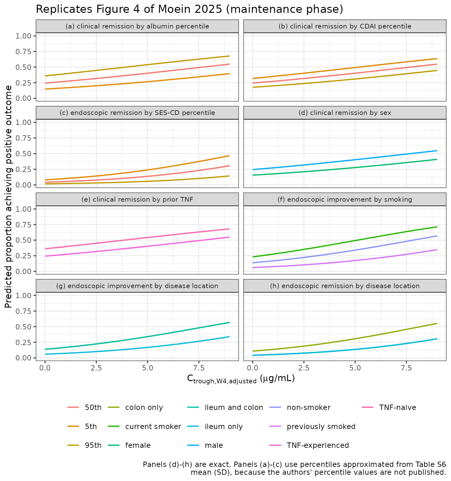
The paper’s headline finding, reproduced
Exposure-response is far more evident at end of maintenance than at end of induction. Over the observed exposure range the maintenance slopes move the predicted response substantially while the induction slopes barely move it.
span <- function(key) {
  lo <- er_solve(key, list(CTROUGH = 0))
  hi <- er_solve(key, list(CTROUGH = 9))
  c(lo = lo, hi = hi, delta = hi - lo)
}
spans <- vapply(names(er_mods), span, c(lo = 0, hi = 0, delta = 0))

tibble::tibble(
  Model = colnames(spans),
  `P at 0 ug/mL` = round(spans["lo", ], 3),
  `P at 9 ug/mL` = round(spans["hi", ], 3),
  `Absolute increase` = round(spans["delta", ], 3),
  `Slope (LO per ug/mL)` = c(0.0259, 0.0682, 0.0495, 0.147, 0.234, 0.257),
  `P-value` = c(0.426, 0.061, 0.297, 0.00544, 0.00012, 0.000555)
) |>
  knitr::kable(
    caption = paste0(
      "Exposure-response span over 0-9 ug/mL. Slopes and P-values are ",
      "Moein 2025 Table 2."
    )
)| Model | P at 0 ug/mL | P at 9 ug/mL | Absolute increase | Slope (LO per ug/mL) | P-value |
|---|---|---|---|---|---|
| induction_clinrem | 0.233 | 0.277 | 0.044 | 0.0259 | 0.426000 |
| induction_endoimp | 0.144 | 0.237 | 0.093 | 0.0682 | 0.061000 |
| induction_endorem | 0.058 | 0.087 | 0.030 | 0.0495 | 0.297000 |
| maintenance_clinrem | 0.244 | 0.548 | 0.304 | 0.1470 | 0.005440 |
| maintenance_endoimp | 0.138 | 0.568 | 0.430 | 0.2340 | 0.000120 |
| maintenance_endorem | 0.042 | 0.306 | 0.264 | 0.2570 | 0.000555 |
# Every maintenance endpoint must gain more from exposure than its induction
# counterpart. This is the paper's central claim and it is a deterministic
# consequence of the published slopes, so it can be asserted exactly.
d <- spans["delta", ]
stopifnot(
  d[["maintenance_clinrem"]] > d[["induction_clinrem"]],
  d[["maintenance_endoimp"]] > d[["induction_endoimp"]],
  d[["maintenance_endorem"]] > d[["induction_endorem"]]
)
End-to-end: population PK feeding the ER models
The two layers compose the way the paper composes them – the population PK model predicts each subject’s week-4 trough after a single dose, and that value is the ER models’ exposure covariate.
er_cohort <- sim_sd |>
  filter(!is.na(Cc), abs(time - 28) < 1e-8) |>
  transmute(id, CTROUGH = Cc) |>
  mutate(
    PRIOR_TNF = rbinom(n(), 1, 0.59), SEXF = rbinom(n(), 1, 0.50),
    ALB = 42.0, SCORE_CDAI = 320, SCORE_SESCD = 12.0,
    DISLOC_ILEUM = 0L, DISLOC_COLON = 0L,
    SMOKE_NEVER = 1L, SMOKE_CURRENT = 0L, time = 0, amt = 0, evid = 0L
  )

pred <- as.data.frame(
  rxode2::rxSolve(er_mods[["maintenance_clinrem"]], events = er_cohort,
                  keep = c("CTROUGH"))
)
#> Warning: multi-subject simulation without without 'omega'

ggplot(pred, aes(x = CTROUGH, y = prob_clinrem)) +
  geom_point(alpha = 0.35, size = 1, colour = "#4682b4") +
  coord_cartesian(ylim = c(0, 1)) +
  labs(
    x = expression("Model-predicted " * C[trough * ",W4"] * " (" * mu * "g/mL)"),
    y = "P(clinical remission at maintenance)",
    title = "Population PK model feeding the maintenance ER model",
    caption = paste0(
      "Each point is one virtual subject: their single-dose week-4 trough ",
      "from the popPK model,\nand the resulting remission probability. The ",
      "two visible bands are TNF-naive vs TNF-experienced."
    )
  ) +
  theme_bw()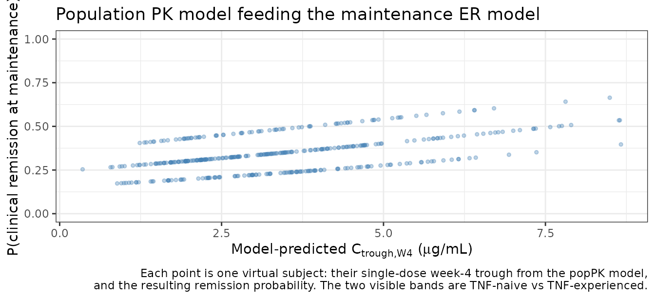
Assumptions and deviations
- Body-weight exponents follow Table 1, not the Results prose. The prose transposes them; Figure 1 discriminates decisively in favour of the table. See the Errata section and the second assertion of gate 1.
-
The phase I/II residual-error covariate is not
implemented. Table 1 retains a -23.0% fractional change on the
overall residual error for phase I/II studies, which rxode2’s error DSL
cannot express. The model carries the phase 3 residual error (the
reference stratum, and the only stratum a Crohn’s-disease simulation can
occupy). The coefficient and a reconstruction recipe are preserved in
the model’s
covariatesDataExcludedentry. -
SCORE_SESCDmust be set to 12 for ulcerative-colitis subjects. SES-CD is recorded only in Crohn’s patients; Moein 2025 assigns UC subjects the reference value so the centred effect cancels. Simulating a UC subject with a different value silently applies a Crohn’s-specific covariate to them. - ADA titer is a cumulative maximum carried forward, not an instantaneous titer (Table 1 footnote d), and is 0 on the linear-titer convention for ADA-negative subjects. The virtual cohorts above use 0 throughout, matching the Figure 1 reference patient (“ADA negative at least until Week 4”).
-
Figure 4 panels (a)-(c) are indicative, not exact.
They stratify on 5th / 50th / 95th percentiles of albumin, CDAI and
SES-CD that the paper does not publish; Table S6 gives mean (SD) and
median (min, max) only. The percentiles used here are
mean +/- 1.645 SDfrom the maintenance column, clamped to the observed range. The SES-CD 5th percentile so computed (1.9) falls below the observed minimum, so it is clamped to 3.0. Panels (d)-(h) need no percentiles and are exact – they carry gate 5. - The Table S6 exposure comparison is soft and ungated. The published distribution pools placebo, 105 mg and 210 mg subjects; the simulated column is 105 mg only. The wide bound in that chunk exists to catch a unit or dose error, not to pin the value.
- Virtual covariate distributions are approximations. Exact joint baseline distributions are not published. The cohort draws marginals matching Tables S6 and S7 (log-normal weight, normal albumin and GFR, log-normal CRP, normal SES-CD, binomial prior anti-TNF) and treats them as independent, which they are not in reality.
-
The ER models carry a placeholder residual. The
source likelihood is Bernoulli and estimates no residual error, but
rxode2 requires an observation declaration, so each ER model fixes a
tiny additive SD (
fixed(0.001)) purely to satisfy the parser. It is not a source value. Draw binary outcomes withrbinom(n, 1, prob_<endpoint>)on the solved probability rather than treating the placeholder as noise. -
Two ER coefficients are structural zeros, not
estimates:
e_colon_endoimpande_ileum_endoremarefixed(0)because the source models did not retain those terms and the Figure 4 caption states the corresponding curves are predicted identically to the reference. -
New canonical names registered with this
extraction.
SCORE_SESCD,DISLOC_ILEUMandDISLOC_COLONwere ratified by the maintainers as general-scope covariate canonicals, andprob_clinrem,prob_endoimpandprob_endoremwere registered as output-state canonicals in the established, explicitly extensibleprob_<endpoint>family.
Reference
- Moein A, Ribbing J, Ibrahim MMA, Zhang W, Kassir N. Population pharmacokinetics and exposure-response relationships of etrolizumab in patients with moderately-to-severely active Crohn’s disease. J Clin Pharmacol. 2025;65(10):1208-1219. doi:10.1002/jcph.70043. Parameter estimates from Table 1; the time-dependent clearance is Equation 1 and Table 1 footnote c; covariate forms are Table 1 footnotes a, b, d and g; the covariate-effect magnitudes were independently confirmed against the fourteen printed ratios of the Figure 1 forest plot. Predecessor UC-only model: Moein A, Lu T, Jonsson S, et al. CPT Pharmacometrics Syst Pharmacol. 2022;11(9):1244-1255. doi:10.1002/psp4.12846; see modellib(‘Moein_2022_etrolizumab’).