Dolutegravir placental and breast-milk transfer (Dickinson 2021)
Source:vignettes/articles/Dickinson_2021_dolutegravir.Rmd
Dickinson_2021_dolutegravir.RmdModel and source
Dickinson et al. (2021) describe dolutegravir in four matrices from the DolPHIN-1 trial, in which women diagnosed with HIV late in pregnancy were randomized to dolutegravir-based therapy: maternal plasma (third trimester, delivery and postpartum), umbilical cord, breast milk, and the plasma of their breastfed infants. The paper builds two models, and the library ships both:
Dickinson_2021_dolutegravir– the maternal model, fitted simultaneously to maternal plasma, cord and breast-milk concentrations.Dickinson_2021_dolutegravir_motherinfant– the infant model, fitted sequentially with the maternal parameters fixed. It carries the complete maternal model plus a one-compartment infant.Citation: Dickinson L, Walimbwa S, Singh Y, Kaboggoza J, Kintu K, Sihlangu M, Coombs JA, Malaba TR, Byamugisha J, Pertinez H, Amara A, Gini J, Else L, Heiberg C, Hodel EM, Reynolds H, Myer L, Waitt C, Khoo S, Lamorde M, Orrell C; DolPHIN-1 Study Group. Infant exposure to dolutegravir through placental and breast milk transfer: a population pharmacokinetic analysis of DolPHIN-1. Clin Infect Dis. 2021;73(5):e1200-e1207. doi:10.1093/cid/ciaa1861. Structure from the Results text and Figure 3; parameter values from Table 2 and its footnote b; estimation and BLQ methods from the Supplementary Material.
Maternal model: Maternal population PK model for oral dolutegravir in women living with HIV who started treatment late in pregnancy (DolPHIN-1), fitted simultaneously to maternal plasma (third trimester, delivery and postpartum), umbilical cord and breast-milk concentrations. Two-compartment disposition with first-order absorption; the maternal central compartment is linked by first-order rate constants to a fetal (umbilical cord) compartment of negligible volume that does not deplete the mother, and to a breast-milk compartment of fixed 0.125 L volume. No covariates were retained. The breastfed-infant extension is modellib(‘Dickinson_2021_dolutegravir_motherinfant’).
Mother-infant model: Mother-to-infant population PK model for dolutegravir (DolPHIN-1), extending the maternal model of modellib(‘Dickinson_2021_dolutegravir’) with a one-compartment breastfed-infant model fitted sequentially with the maternal parameters fixed. At delivery the infant is born with the transplacental amount on board, equal to the predicted umbilical-cord concentration times the mother’s apparent central volume; thereafter the infant receives dolutegravir by first-order input from the mother’s breast-milk compartment and eliminates it by a first-order infant elimination rate constant. The time-varying PREG indicator marks delivery: while PREG = 1 the infant state tracks the transplacental amount, and from the first PREG = 0 record the infant ODE runs.
Article: https://doi.org/10.1093/cid/ciaa1861 (open access; the Supplementary Material gives the estimation, BLQ and covariate methods).
Population
The maternal model was fitted to 28 women (14 in Kampala, Uganda and 14 in Cape Town, South Africa) aged 19-42 years (median 27) weighing 44-160 kg (median 67). They started dolutegravir 50 mg once daily at 28-36 weeks’ gestation and were sampled intensively over 24 h on day 14 of treatment (third trimester), at delivery (with a paired cord sample) and within 1-3 weeks after delivery, after which they were switched to efavirenz-based therapy and mother and infant were sampled up to 96 h after the final dolutegravir dose. The postpartum sampling interval was a median of 7 days (range 2-18). The data comprised 533 maternal plasma, 16 cord and 80 breast-milk concentrations.
The infant model was fitted to 65 plasma concentrations from 22
breastfed infants with a recorded delivery time: 17 boys and 5 girls,
birth weight 3.3 kg (2.5-4.3), gestational age 39 weeks (35-43),
postnatal age 7 days (3-18) (Table 1). The same information is available
programmatically via
readModelDb("Dickinson_2021_dolutegravir")()$population and
readModelDb("Dickinson_2021_dolutegravir_motherinfant")()$population.
Source trace
| Equation / parameter | Value | Source location |
|---|---|---|
| Two-compartment maternal model, first-order absorption | n/a | Results, ‘Population Pharmacokinetic Modeling’; Figure 3 |
lcl (CL/F) |
1.50 L/h | Table 2 |
lvc (Vc/F) |
24.6 L | Table 2 |
lq (Q/F) |
0.0138 L/h | Table 2 |
lvp (Vp/F) |
2.01 L | Table 2 |
lka |
0.75 1/h | Table 2 |
| Fetal compartment of negligible volume, not altering the mother | n/a | Results text; Figure 3 |
lk_central_fetal (kM-F) |
2.81 1/h | Table 2 |
lk_fetal_central (kF-M) |
2.20 1/h | Table 2 |
| Breast-milk compartment linked to maternal central | n/a | Results text; Figure 3 |
lk_central_milk (kM-BM) |
0.0027 1/h | Table 2 |
lk_milk_central (kBM-M) |
16.3 1/h | Table 2 |
lvmilk (VBM) |
0.125 L, fixed | Table 2; Results (refs 16 and 18) |
| Infant: one compartment, transplacental initial amount + breast-milk input | n/a | Results text; Figure 3; Supplementary Material |
| Transplacental amount = cord concentration at delivery x maternal Vc/F | n/a | Results, ‘Patients and Pharmacokinetic Sampling’; Supplementary Material |
lkmilkinf (kBM-INF) |
3.22 1/h | Table 2 |
lkel_infant (kINF) |
0.0162 1/h | Table 2 |
lvc_infant (VINF/F) |
30.1 L | Table 2 |
etalcl, etalvc
|
14.3%, 20.7% CV; correlation 0.88 | Table 2 footnote b; Table 2 correlation row |
etaiov_cl_* |
21.0% CV | Table 2 footnote b |
etalkel_infant |
43.6% CV | Table 2 footnote b |
propSd, propSd_Cfetal,
propSd_Cmilk, propSd_Cinfant
|
36.5%, 33.0%, 58.4%, 34.4% | Table 2, ‘Residual error, %’ |
Structural checks on the typical values
Three quantities follow from the typical parameters alone, with no
simulation noise, so they are checked tightly. At steady state the
maternal AUC over a dosing interval is dose / CL/F; because
the fetal compartment is a non-depleting link, the cord:maternal
concentration ratio settles to kM-F / kF-M; and the
milk:maternal ratio is (kM-BM / kBM-M) x (Vc/F / VBM). The
paper reports the last two as model ratios of 1.279 and 0.033.
mod_mat <- readModelDb("Dickinson_2021_dolutegravir")
mod_mi <- readModelDb("Dickinson_2021_dolutegravir_motherinfant")

dose_times <- seq(0, 24 * 27, by = 24)
ev_typ <- dplyr::bind_rows(
  data.frame(id = 1L, time = dose_times, amt = 50, evid = 1L, cmt = "depot", dvid = NA_integer_),
  data.frame(id = 1L, time = seq(0, 24 * 28, by = 0.25), amt = 0, evid = 0L, cmt = "central", dvid = 1L)
) |>
  dplyr::arrange(time, dplyr::desc(evid)) |>
  dplyr::mutate(OCC = 1L, PREG = 1L)

sim_typ <- rxode2::rxSolve(
  rxode2::zeroRe(mod_mat), ev_typ,
  rtol = 1e-10, atol = 1e-12, returnType = "data.frame"
)
#> ℹ parameter labels from comments will be replaced by 'label()'
#> Warning: some etas defaulted to non-mu referenced, possible parsing error: etaiov_cl_1, etaiov_cl_2, etaiov_cl_3
#> as a work-around try putting the mu-referenced expression on a simple line
#> Warning: some etas defaulted to non-mu referenced, possible parsing error: etaiov_cl_1, etaiov_cl_2, etaiov_cl_3
#> as a work-around try putting the mu-referenced expression on a simple line
#> ℹ omega/sigma items treated as zero: 'etalcl', 'etalvc', 'etaiov_cl_1', 'etaiov_cl_2', 'etaiov_cl_3'
ss_day <- dplyr::filter(sim_typ, time >= 24 * 27, time <= 24 * 28)
trap <- function(x, y) sum(diff(x) * (head(y, -1) + tail(y, -1)) / 2)
auc_ss <- trap(ss_day$time, ss_day$Cc)
ratio_cord <- trap(ss_day$time, ss_day$Cfetal) / auc_ss
ratio_milk <- trap(ss_day$time, ss_day$Cmilk) / auc_ss

typ <- data.frame(
  Quantity = c("Maternal AUC0-24 at steady state (mg*h/L)", "Cord:maternal AUC ratio", "Breast milk:maternal AUC ratio"),
  Expected = c(50 / 1.50, 2.81 / 2.20, (0.0027 / 16.3) * (24.6 / 0.125)),
  Published = c(NA, 1.279, 0.033),
  Simulated = c(auc_ss, ratio_cord, ratio_milk)
)
knitr::kable(typ, digits = 4, caption = "Typical-value structural checks after 28 days of 50 mg once daily.")| Quantity | Expected | Published | Simulated |
|---|---|---|---|
| Maternal AUC0-24 at steady state (mg*h/L) | 33.3333 | NA | 33.3214 |
| Cord:maternal AUC ratio | 1.2773 | 1.279 | 1.2776 |
| Breast milk:maternal AUC ratio | 0.0326 | 0.033 | 0.0326 |
# The milk compartment exchanges mass with the maternal central compartment,
# which adds (kM-BM / kBM-M) x Vc = 0.004 L to the steady-state volume and
# nothing to the dosing-interval AUC; the 0.25-h trapezoid on the absorption
# peak is the only other error term (measured ~5e-5 relative).
stopifnot(
  abs(auc_ss / (50 / 1.50) - 1) < 1e-3,
  abs(ratio_cord / (2.81 / 2.20) - 1) < 1e-3,
  abs(ratio_milk / ((0.0027 / 16.3) * (24.6 / 0.125)) - 1) < 1e-3,
  # and the model reproduces the published ratios to their printed precision
  abs(ratio_cord - 1.279) < 0.005,
  abs(ratio_milk - 0.033) < 0.001
)

# The mother-infant model carries the identical maternal layer.
sim_typ_mi <- rxode2::rxSolve(
  rxode2::zeroRe(mod_mi), ev_typ,
  rtol = 1e-10, atol = 1e-12, returnType = "data.frame"
)
#> ℹ parameter labels from comments will be replaced by 'label()'
#> Warning: some etas defaulted to non-mu referenced, possible parsing error: etaiov_cl_1, etaiov_cl_2, etaiov_cl_3
#> as a work-around try putting the mu-referenced expression on a simple line
#> Warning: some etas defaulted to non-mu referenced, possible parsing error: etaiov_cl_1, etaiov_cl_2, etaiov_cl_3
#> as a work-around try putting the mu-referenced expression on a simple line
#> ℹ omega/sigma items treated as zero: 'etalcl', 'etalvc', 'etaiov_cl_1', 'etaiov_cl_2', 'etaiov_cl_3', 'etalkel_infant'
stopifnot(
  max(abs(sim_typ_mi$Cc - sim_typ$Cc)) < 1e-8,
  max(abs(sim_typ_mi$Cmilk - sim_typ$Cmilk)) < 1e-8,
  max(abs(sim_typ_mi$Cfetal - sim_typ$Cfetal)) < 1e-8
)
Virtual cohort
Observed data are not public. The cohort below reproduces the DolPHIN-1 timeline: dolutegravir 50 mg every morning for 28 days before delivery (so the day-14 third-trimester profile and delivery are both well past steady state), delivery at a uniformly distributed time within a dosing interval, and a final maternal dose on postpartum day 2-18 drawn from the Table 1 distribution of postpartum sampling intervals (56% within 1 week, 33% within 2 weeks, 11% within 3 weeks). Mothers and infants are followed for 240 h after the final maternal dose.
# `set.seed()` seeds R's RNG (used for the delivery and stopping times).
# rxode2's own simulation RNG is set by rxSetSeed(), and its streams are
# partitioned per solver thread, so the cohort differs between machines with
# different thread counts. Every assertion below is written on the centre of
# the distribution for that reason.
set.seed(2021)
rxode2::rxSetSeed(2021)

n_sub <- 200L
# Postpartum day of the final maternal dose: Table 1 bins (within 1, 2 and
# 3 weeks), uniform within each bin, range 2-18 days as reported.
pp_bins <- list(2:7, 8:14, 15:18)
pp_bin <- sample(1:3, n_sub, replace = TRUE, prob = c(0.56, 0.33, 0.11))
pp_days <- vapply(pp_bins[pp_bin], function(b) sample(b, 1), integer(1))

subj <- tibble::tibble(
  id = seq_len(n_sub),
  t_del = 24 * 28 + runif(n_sub, 0, 24),
  pp_day = pp_days
) |>
  dplyr::mutate(t_last = 24 * (28 + pp_day))

make_events <- function(s) {
  doses <- seq(0, s$t_last, by = 24)
  obs <- sort(unique(c(
    24 * 14 + seq(0, 24, by = 1), # third-trimester intensive profile
    s$t_del, # delivery (paired maternal and cord sample)
    seq(ceiling(s$t_del), s$t_last, by = 6), # postpartum
    s$t_last + c(seq(0, 96, by = 1), seq(98, 240, by = 2)) # after the final dose
  )))
  dplyr::bind_rows(
    data.frame(time = doses, amt = 50, evid = 1L, cmt = "depot", dvid = NA_integer_),
    data.frame(time = obs, amt = 0, evid = 0L, cmt = "central", dvid = 1L)
  ) |>
    dplyr::mutate(
      id = s$id, t_del = s$t_del, t_last = s$t_last, pp_day = s$pp_day,
      PREG = as.integer(time < s$t_del),
      # occasion 1 = antepartum, occasion 3 = postpartum (see Assumptions)
      OCC = ifelse(time < s$t_del, 1L, 3L)
    )
}

events <- dplyr::bind_rows(lapply(split(subj, subj$id), make_events)) |>
  dplyr::arrange(id, time, dplyr::desc(evid))
stopifnot(!anyDuplicated(events[, c("id", "time", "evid")]))
Simulation
sim <- rxode2::rxSolve(
  mod_mi, events,
  keep = c("t_del", "t_last", "pp_day"),
  returnType = "data.frame"
)
#> ℹ parameter labels from comments will be replaced by 'label()'
#> Warning: some etas defaulted to non-mu referenced, possible parsing error: etaiov_cl_1, etaiov_cl_2, etaiov_cl_3
#> as a work-around try putting the mu-referenced expression on a simple line
stopifnot(!anyNA(sim$Cc), !anyNA(sim$Cinfant))

# Individual infant elimination rate constants, for the half-life summary.
indiv <- sim |>
  dplyr::group_by(id) |>
  dplyr::slice(1) |>
  dplyr::ungroup() |>
  dplyr::transmute(id, vc, kel_infant, t_half_infant = log(2) / kel_infant)
The transplacental dose
Before delivery the infant state tracks the cord concentration times the mother’s apparent central volume; at delivery that amount is the infant’s initial condition. The check below confirms the identity on every simulated subject, then compares the resulting doses with the paper’s median of 39.9 mg (range 15.5-59.0 mg).
at_del <- sim |>
  dplyr::filter(abs(time - t_del) < 1e-9) |>
  dplyr::left_join(indiv |> dplyr::select(id, vc_i = vc), by = "id") |>
  dplyr::mutate(dose_tp = Cfetal * vc_i, ratio_cord_mat = Cfetal / Cc)
stopifnot(
  nrow(at_del) == n_sub,
  max(abs(at_del$infant_central / at_del$dose_tp - 1)) < 1e-4
)
summary_tp <- data.frame(
  Quantity = c("Transplacental infant dose (mg)", "Cord:maternal concentration ratio at delivery"),
  Published = c("39.9 (15.5-59.0)", "1.279 (1.209-1.281), as a 0-24 h AUC ratio"),
  Simulated = c(
    sprintf("%.1f (%.1f-%.1f)", median(at_del$dose_tp), min(at_del$dose_tp), max(at_del$dose_tp)),
    sprintf("%.3f (%.3f-%.3f)", median(at_del$ratio_cord_mat), min(at_del$ratio_cord_mat), max(at_del$ratio_cord_mat))
  )
)
knitr::kable(summary_tp, caption = "Median (range) at delivery.")| Quantity | Published | Simulated |
|---|---|---|
| Transplacental infant dose (mg) | 39.9 (15.5-59.0) | 44.0 (11.4-88.3) |
| Cord:maternal concentration ratio at delivery | 1.279 (1.209-1.281), as a 0-24 h AUC ratio | 1.309 (0.766-1.348) |
# Transplacental dose: a mis-transcribed kM-F, kF-M or Vc/F moves the median
# by tens of percent; the random delivery time within the dosing interval and
# Vc/F IIV set the spread.
stopifnot(abs(median(at_del$dose_tp) / 39.9 - 1) < 0.25)
The cord:maternal concentration ratio at a single time is
not constant: it lags behind the maternal profile by the fetal
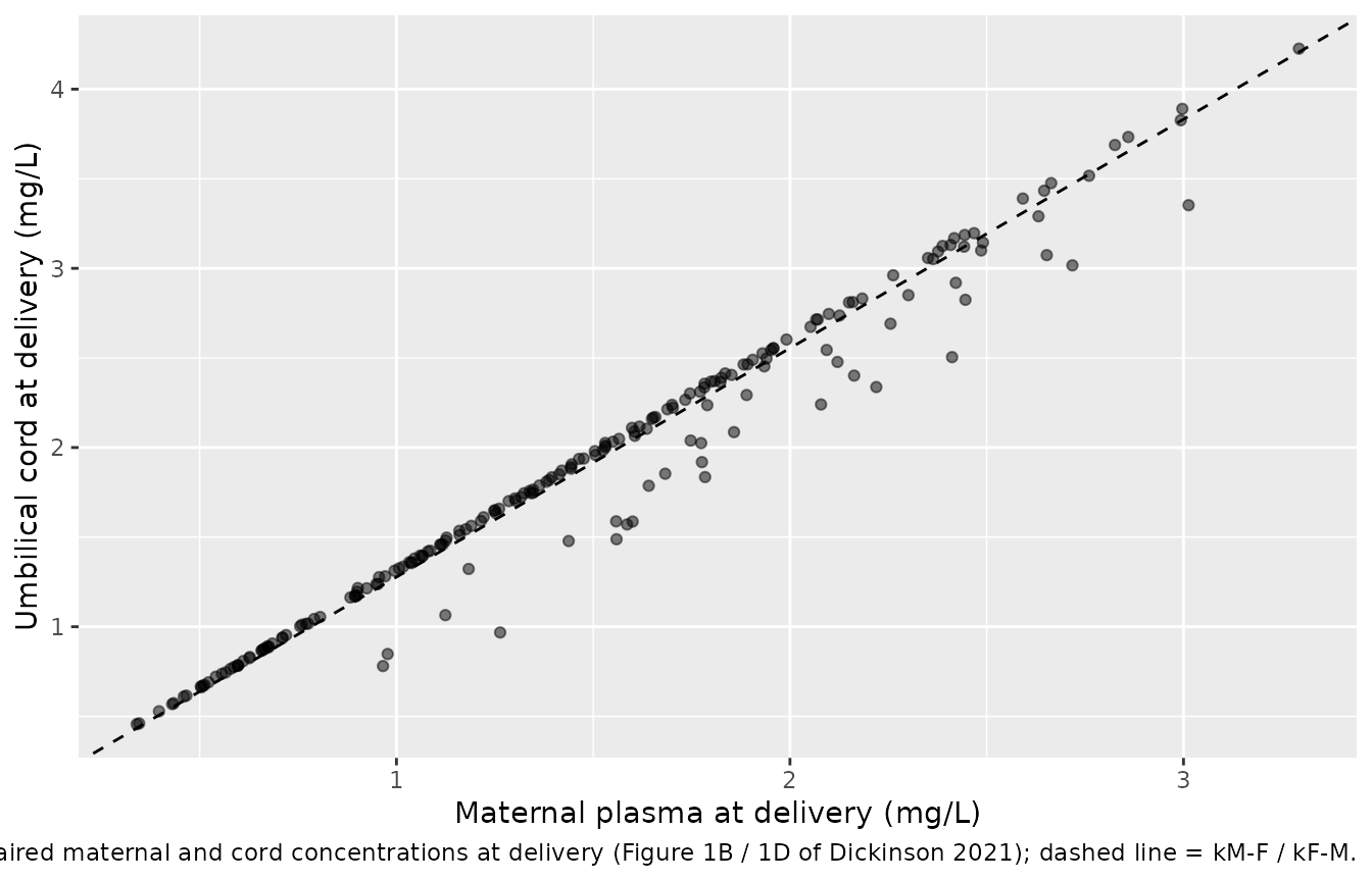
equilibration half-life of log(2) / 2.20 = 0.3 h, so it is
below the steady-state value of 1.277 while maternal concentrations rise
after a dose and above it while they fall. The AUC ratio above is the
quantity the paper summarises.
Replicate published figures
Figure 1 – maternal plasma, cord and breast milk
pct <- function(d, x, y) {
  d |>
    dplyr::group_by(.data[[x]]) |>
    dplyr::summarise(
      Q05 = quantile(.data[[y]], 0.05),
      Q50 = quantile(.data[[y]], 0.50),
      Q95 = quantile(.data[[y]], 0.95),
      .groups = "drop"
    ) |>
    dplyr::rename(tad = !!x)
}

third <- sim |>
  dplyr::filter(time >= 24 * 14, time <= 24 * 15) |>
  dplyr::mutate(tad = time - 24 * 14)
post <- sim |>
  dplyr::filter(time >= t_last, time <= t_last + 96) |>
  dplyr::mutate(tad = round(time - t_last, 6))

fig1 <- dplyr::bind_rows(
  pct(third, "tad", "Cc") |> dplyr::mutate(panel = "A. Maternal plasma, third trimester"),
  pct(post, "tad", "Cc") |> dplyr::mutate(panel = "C. Maternal plasma after the final dose"),
  pct(post, "tad", "Cmilk") |> dplyr::mutate(panel = "E. Breast milk after the final dose")
)
ggplot(fig1, aes(tad, Q50)) +
  geom_ribbon(aes(ymin = Q05, ymax = Q95), alpha = 0.25) +
  geom_line() +
  geom_hline(yintercept = 0.01, linetype = "dotted") +
  facet_wrap(~panel, scales = "free_x", ncol = 2) +
  scale_y_log10() +
  labs(
    x = "Time after dose (h)", y = "Dolutegravir (mg/L)",
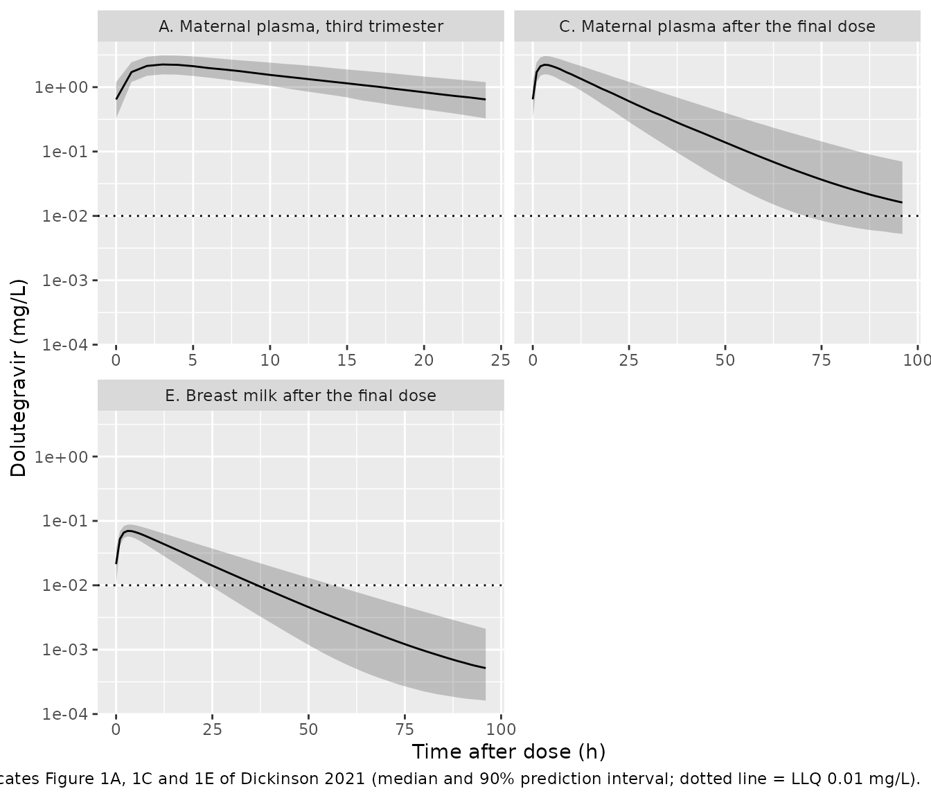
    caption = "Replicates Figure 1A, 1C and 1E of Dickinson 2021 (median and 90% prediction interval; dotted line = LLQ 0.01 mg/L)."
  )
ggplot(at_del, aes(Cc, Cfetal)) +
  geom_point(alpha = 0.5) +
  geom_abline(slope = 2.81 / 2.20, linetype = "dashed") +
  labs(
    x = "Maternal plasma at delivery (mg/L)", y = "Umbilical cord at delivery (mg/L)",
    caption = "Paired maternal and cord concentrations at delivery (Figure 1B / 1D of Dickinson 2021); dashed line = kM-F / kF-M."
  )
Breast-milk concentrations fall below the 0.01 mg/L LLQ within about two days of the final dose, in line with the paper’s report that milk dolutegravir was undetectable in 88.9% of samples 46-50 h and all samples from 71 h after the switch.
Figure 2 – infant plasma after the final maternal dose
inf_post <- sim |>
  dplyr::filter(time >= t_last, time <= t_last + 100) |>
  dplyr::mutate(tad = round(time - t_last, 6))
pct(inf_post, "tad", "Cinfant") |>
  ggplot(aes(tad, Q50)) +
  geom_ribbon(aes(ymin = Q05, ymax = Q95), alpha = 0.25) +
  geom_line() +
  scale_y_log10(limits = c(0.001, 10)) +
  labs(
    x = "Time after the final maternal dose (h)", y = "Infant dolutegravir (mg/L)",
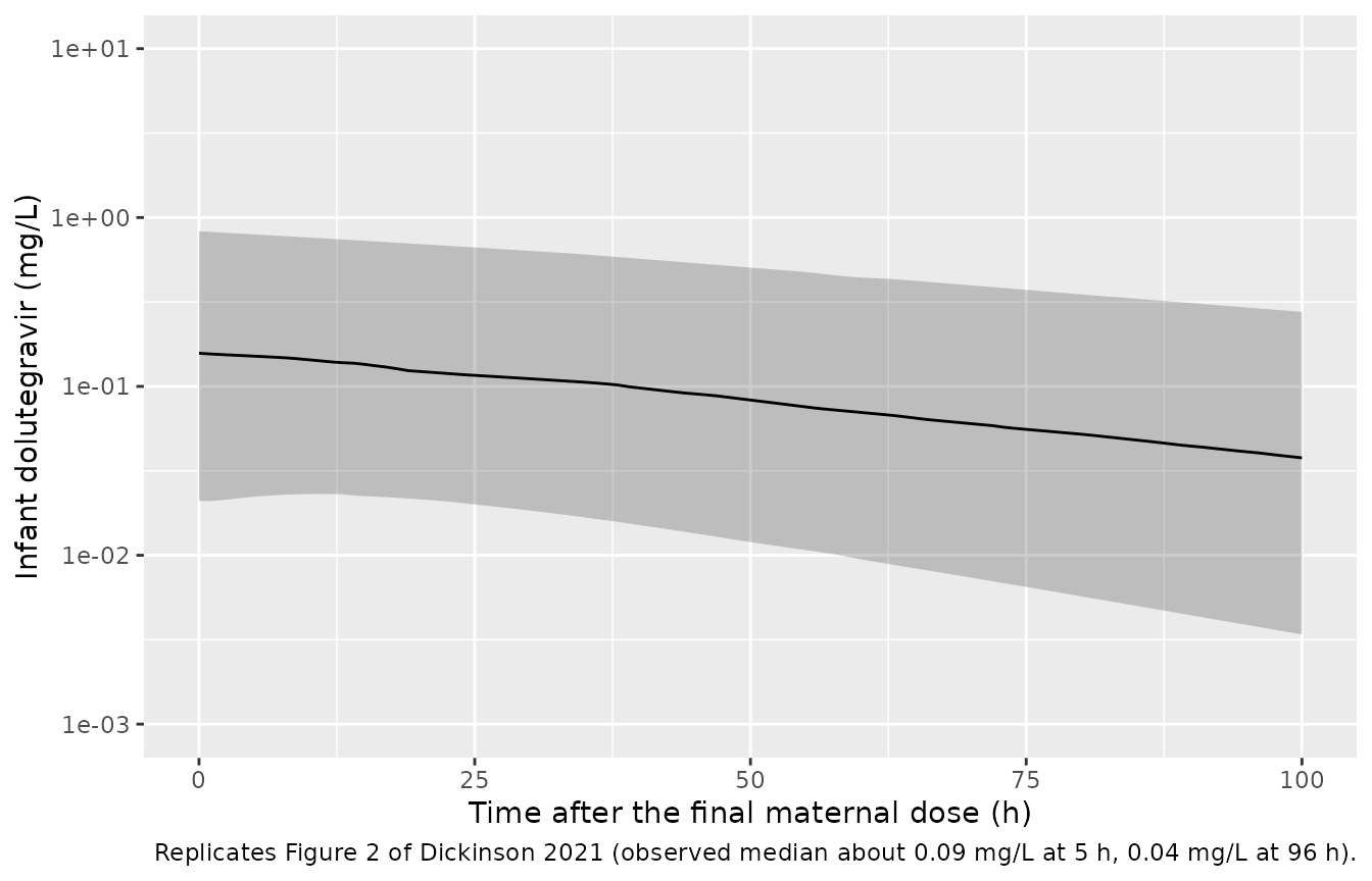
    caption = "Replicates Figure 2 of Dickinson 2021 (observed median about 0.09 mg/L at 5 h, 0.04 mg/L at 96 h)."
  )
inf_med <- inf_post |>
  dplyr::filter(tad %in% c(4, 96)) |>
  dplyr::group_by(tad) |>
  dplyr::summarise(median_Cinfant = median(Cinfant), .groups = "drop")
knitr::kable(inf_med, digits = 3, caption = "Simulated median infant concentration after the final maternal dose.")| tad | median_Cinfant |
|---|---|
| 4 | 0.152 |
| 96 | 0.040 |
PKNCA validation
Table 3 of the paper gives individual-prediction AUCs over 24, 48, 72 and 96 h after the final maternal dose, in maternal plasma, breast milk and infant plasma; the Discussion adds the geometric-mean predicted maternal AUC0-24 in the third trimester (33.0 mg*h/L). Time is re-based to the dose that starts each window.
nca_long <- dplyr::bind_rows(
  third |> dplyr::transmute(id, tad, conc = Cc, matrix = "Maternal plasma, third trimester"),
  post |> dplyr::transmute(id, tad, conc = Cc, matrix = "Maternal plasma"),
  post |> dplyr::transmute(id, tad, conc = Cmilk, matrix = "Breast milk"),
  inf_post |> dplyr::filter(tad <= 96) |> dplyr::transmute(id, tad, conc = Cinfant, matrix = "Infant plasma")
) |>
  dplyr::filter(!is.na(conc)) |>
  dplyr::distinct(id, matrix, tad, .keep_all = TRUE) |>
  dplyr::arrange(matrix, id, tad)
stopifnot(all(dplyr::summarise(dplyr::group_by(nca_long, matrix, id), t0 = min(tad))$t0 == 0))
#> `summarise()` has regrouped the output.
#> ℹ Summaries were computed grouped by matrix and id.
#> ℹ Output is grouped by matrix.
#> ℹ Use `summarise(.groups = "drop_last")` to silence this message.
#> ℹ Use `summarise(.by = c(matrix, id))` for per-operation grouping
#>   (`?dplyr::dplyr_by`) instead.

run_nca <- function(mx, ends) {
  d <- dplyr::filter(nca_long, matrix == mx)
  dose <- dplyr::distinct(d, id, matrix) |> dplyr::mutate(tad = 0, amt = 50)
  intervals <- data.frame(start = 0, end = ends, auclast = TRUE)
  res <- PKNCA::pk.nca(PKNCA::PKNCAdata(
    PKNCA::PKNCAconc(d, conc ~ tad | matrix + id),
    PKNCA::PKNCAdose(dose, amt ~ tad | matrix + id),
    intervals = intervals
  ))
  as.data.frame(res) |>
    dplyr::mutate(window = paste0("AUC0-", end)) |>
    dplyr::select(id, matrix, window, PPTESTCD, PPORRES)
}

nca_sim <- dplyr::bind_rows(
  run_nca("Maternal plasma, third trimester", 24),
  run_nca("Maternal plasma", c(24, 48, 72, 96)),
  run_nca("Breast milk", c(24, 48, 72, 96)),
  run_nca("Infant plasma", c(24, 48, 72, 96))
)
Comparison against published values
published <- tibble::tribble(
  ~matrix, ~window, ~auclast,
  "Maternal plasma, third trimester", "AUC0-24", 33.0,
  "Maternal plasma", "AUC0-24", 38.0,
  "Maternal plasma", "AUC0-48", 49.8,
  "Maternal plasma", "AUC0-72", 52.0,
  "Maternal plasma", "AUC0-96", 52.7,
  "Breast milk", "AUC0-24", 1.20,
  "Breast milk", "AUC0-48", 1.56,
  "Breast milk", "AUC0-72", 1.66,
  "Breast milk", "AUC0-96", 1.68,
  "Infant plasma", "AUC0-24", 1.87,
  "Infant plasma", "AUC0-48", 3.48,
  "Infant plasma", "AUC0-72", 4.76,
  "Infant plasma", "AUC0-96", 5.45
)

cmp <- nlmixr2lib::ncaComparisonTable(
  simulated = dplyr::select(nca_sim, -id),
  reference = published,
  by = c("matrix", "window"),
  units = c(auclast = "mg*h/L"),
  tolerance_pct = 20
)
knitr::kable(
  cmp,
  caption = "Simulated median vs published (Table 3 medians; third-trimester value is the Discussion's geometric mean). * differs by >20%."
)| NCA parameter | matrix | window | Reference | Simulated | % diff |
|---|---|---|---|---|---|
| AUClast (mg*h/L) | Maternal plasma, third trimester | AUC0-24 | 33 | 33 | -0.1% |
| AUClast (mg*h/L) | Maternal plasma | AUC0-24 | 38 | 33.7 | -11.2% |
| AUClast (mg*h/L) | Maternal plasma | AUC0-48 | 49.8 | 41.7 | -16.3% |
| AUClast (mg*h/L) | Maternal plasma | AUC0-72 | 52 | 43.4 | -16.4% |
| AUClast (mg*h/L) | Maternal plasma | AUC0-96 | 52.7 | 44.2 | -16.1% |
| AUClast (mg*h/L) | Breast milk | AUC0-24 | 1.2 | 1.07 | -10.6% |
| AUClast (mg*h/L) | Breast milk | AUC0-48 | 1.56 | 1.35 | -13.8% |
| AUClast (mg*h/L) | Breast milk | AUC0-72 | 1.66 | 1.41 | -14.9% |
| AUClast (mg*h/L) | Breast milk | AUC0-96 | 1.68 | 1.43 | -14.6% |
| AUClast (mg*h/L) | Infant plasma | AUC0-24 | 1.87 | 3.36 | +79.5%* |
| AUClast (mg*h/L) | Infant plasma | AUC0-48 | 3.48 | 5.63 | +61.9%* |
| AUClast (mg*h/L) | Infant plasma | AUC0-72 | 4.76 | 7.6 | +59.7%* |
| AUClast (mg*h/L) | Infant plasma | AUC0-96 | 5.45 | 9.06 | +66.3%* |
sim_med <- nca_sim |>
  dplyr::group_by(matrix, window) |>
  dplyr::summarise(sim = median(PPORRES), .groups = "drop") |>
  dplyr::inner_join(published, by = c("matrix", "window")) |>
  dplyr::mutate(pct = 100 * (sim / auclast - 1))
stopifnot(nrow(sim_med) == nrow(published))

# Maternal plasma and milk are gated on what the typical parameters imply
# (dose / CL/F = 33.3 mg*h/L at steady state, and the typical milk:maternal
# ratio), not on the published postpartum medians: those are individual
# predictions for the 27 DolPHIN-1 mothers, whose CL/F ran below the typical
# value (their postpartum AUC0-24 of 38.0 exceeds dose / CL/F), so any
# typical-parameter cohort sits 10-17% below them. A mis-transcribed CL/F,
# Vc/F, kM-BM, kBM-M or VBM moves these medians by tens of percent; the
# cohort median itself moves by about 2% between draws (CV about 25% on
# AUC0-24, n = 200).
auc_typ <- 50 / 1.50
med_of <- function(mx, w) sim_med$sim[sim_med$matrix == mx & sim_med$window == w]
stopifnot(
  abs(med_of("Maternal plasma, third trimester", "AUC0-24") / auc_typ - 1) < 0.1,
  abs(med_of("Maternal plasma", "AUC0-24") / auc_typ - 1) < 0.1,
  abs(med_of("Breast milk", "AUC0-24") / (ratio_milk * auc_typ) - 1) < 0.1
)
The maternal and breast-milk rows reproduce Table 3 to within 17%, with the simulated values uniformly 10-17% low for the reason given in the code comment.
The infant rows are not reproduced: the simulated medians are 60-80% above Table 3. Transcription of the four infant quantities (kBM-INF, kINF, VINF/F and the transplacental-dose rule) was re-checked against Table 2 and the Supplementary Material. The typical-value sensitivity below, for an infant whose mother stops dolutegravir on postpartum day 7 after a delivery 12 h after a dose, shows where the difference can and cannot come from.
# The parser note about non-mu-referenced IOV etas is cosmetic; the etas are
# zeroed here anyway.
mod_mi_typ <- rxode2::zeroRe(mod_mi)
sens_run <- function(label, pars) {
  t_del <- 24 * 28 + 12
  t_last <- 24 * (28 + 7)
  obs <- sort(unique(c(t_del, t_last + seq(0, 96, by = 0.5))))
  ev <- dplyr::bind_rows(
    data.frame(time = seq(0, t_last, by = 24), amt = 50, evid = 1L, cmt = "depot", dvid = NA_integer_),
    data.frame(time = obs, amt = 0, evid = 0L, cmt = "central", dvid = 1L)
  ) |>
    dplyr::arrange(time, dplyr::desc(evid)) |>
    dplyr::mutate(id = 1L, PREG = as.integer(time < t_del), OCC = ifelse(time < t_del, 1L, 3L))
  s <- rxode2::rxSolve(mod_mi_typ, ev, params = pars, returnType = "data.frame")
  p <- dplyr::filter(s, time >= t_last) |> dplyr::mutate(t = time - t_last)
  auc_to <- function(e) with(dplyr::filter(p, t <= e), trap(t, Cinfant))
  data.frame(
    Scenario = label,
    `C at 4 h (mg/L)` = p$Cinfant[p$t == 4],
    `C at 96 h (mg/L)` = p$Cinfant[p$t == 96],
    `AUC0-24` = auc_to(24), `AUC0-48` = auc_to(48), `AUC0-72` = auc_to(72), `AUC0-96` = auc_to(96),
    check.names = FALSE
  )
}
sens <- dplyr::bind_rows(
  sens_run("Model as published", c()),
  sens_run("No breast-milk input (transplacental only)", c(lkmilkinf = log(1e-8))),
  sens_run("Milk amount reduced by 16.3 / (16.3 + 3.22), as a draining input would", c(lkmilkinf = log(3.22 * 16.3 / (16.3 + 3.22)))),
  sens_run("kINF at the paper's median individual half-life (37.9 h)", c(lkel_infant = log(log(2) / 37.9))),
  data.frame(
    Scenario = "Published (Table 3 medians; Figure 2 observed medians read by the maintainers)",
    `C at 4 h (mg/L)` = 0.09, `C at 96 h (mg/L)` = 0.037,
    `AUC0-24` = 1.87, `AUC0-48` = 3.48, `AUC0-72` = 4.76, `AUC0-96` = 5.45,
    check.names = FALSE
  )
)
knitr::kable(sens, digits = 3, caption = "Typical-value infant exposure after the final maternal dose on postpartum day 7.")| Scenario | C at 4 h (mg/L) | C at 96 h (mg/L) | AUC0-24 | AUC0-48 | AUC0-72 | AUC0-96 |
|---|---|---|---|---|---|---|
| Model as published | 0.145 | 0.038 | 3.195 | 5.519 | 7.132 | 8.236 |
| No breast-milk input (transplacental only) | 0.111 | 0.025 | 2.359 | 3.958 | 5.042 | 5.777 |
| Milk amount reduced by 16.3 / (16.3 + 3.22), as a draining input would | 0.140 | 0.036 | 3.057 | 5.261 | 6.787 | 7.830 |
| kINF at the paper’s median individual half-life (37.9 h) | 0.110 | 0.025 | 2.420 | 4.134 | 5.275 | 6.021 |
| Published (Table 3 medians; Figure 2 observed medians read by the maintainers) | 0.090 | 0.037 | 1.870 | 3.480 | 4.760 | 5.450 |
The transplacental amount alone already gives an AUC0-24 above the published median, so no reading of the breast-milk transfer can close the gap; the drain-versus-no-drain question moves infant exposure by about 4%. Exposure a week after birth is exponentially sensitive to kINF: at the paper’s median individual half-life of 37.9 h rather than the typical 42.8 h, infant AUC0-24 falls by a quarter. The published values are individual predictions for 21 infants whose delivery times, postpartum stopping days and individual elimination rates are not reported, so the maintainers treat the infant AUC rows as a documented deviation and do not gate on them. The late infant concentration, which by 96 h after the final dose reflects mainly transplacental drug cleared at kINF, is reproduced:
c96 <- inf_post |>
  dplyr::filter(tad == 96) |>
  dplyr::pull(Cinfant)
# Figure 2 observed median about 0.037 mg/L at 96 h (read off the figure by
# the maintainers). With 43.6% IIV on kINF applied over roughly 264 h of
# decline, log(Cinfant) has an SD near 1.9, so the cohort median moves by
# about +/-16% (one SE) between draws; the bound of log(1.65) is 3 SE. A
# ten-fold error in VINF/F or a transposed kINF breaks it.
stopifnot(abs(log(median(c96) / 0.037)) < log(1.65))
Infant half-life and time to the protein-adjusted IC90
The paper reports a median infant half-life of 37.9 h (range 22.1-63.5 h, n = 21 individual estimates) and, for the 13 of 22 infants whose predicted concentration was above the protein-adjusted IC90 of 0.064 mg/L at the final maternal dose, a median time to fall below it of 108.9 h (18.6-129.6 h).
ic90 <- 0.064
t_ic <- inf_post |>
  dplyr::bind_rows(
    sim |> dplyr::filter(time > t_last + 100) |> dplyr::mutate(tad = time - t_last)
  ) |>
  dplyr::arrange(id, tad) |>
  dplyr::group_by(id, pp_day) |>
  dplyr::summarise(
    above0 = Cinfant[tad == 0] > ic90,
    t_below = if (any(Cinfant <= ic90)) min(tad[Cinfant <= ic90]) else NA_real_,
    .groups = "drop"
  )
# Infants still above the threshold 240 h after the final dose (possible for
# a long-half-life draw) are counted but have no crossing time.
n_still_above <- sum(is.na(t_ic$t_below))

ic_tab <- data.frame(
  Quantity = c(
    "Infant half-life, median (range), h",
    "Infants above IC90 at the final maternal dose",
    "Time to fall below IC90 among those, median (range), h",
    "Postpartum day of final dose, above vs below IC90"
  ),
  Published = c("37.9 (22.1-63.5)", "13 of 22 (59%)", "108.9 (18.6-129.6)", "7 (3-15) vs 11 (7-18)"),
  Simulated = c(
    sprintf("%.1f (%.1f-%.1f)", median(indiv$t_half_infant), min(indiv$t_half_infant), max(indiv$t_half_infant)),
    sprintf("%d of %d (%.0f%%)", sum(t_ic$above0), nrow(t_ic), 100 * mean(t_ic$above0)),
    with(
      dplyr::filter(t_ic, above0, !is.na(t_below)),
      sprintf("%.1f (%.1f-%.1f)", median(t_below), min(t_below), max(t_below))
    ),
    sprintf(
      "%.0f vs %.0f",
      median(t_ic$pp_day[t_ic$above0]), median(t_ic$pp_day[!t_ic$above0])
    )
  )
)
knitr::kable(ic_tab, caption = "Infant exposure summaries.")| Quantity | Published | Simulated |
|---|---|---|
| Infant half-life, median (range), h | 37.9 (22.1-63.5) | 43.0 (10.9-147.1) |
| Infants above IC90 at the final maternal dose | 13 of 22 (59%) | 143 of 200 (72%) |
| Time to fall below IC90 among those, median (range), h | 108.9 (18.6-129.6) | 93.0 (1.0-234.0) |
| Postpartum day of final dose, above vs below IC90 | 7 (3-15) vs 11 (7-18) | 5 vs 12 |
n_still_above
#> [1] 10

# The typical infant half-life is log(2) / 0.0162 = 42.8 h, and a lognormal
# kINF has that as its median; the paper's 37.9 h is the median of 21
# empirical Bayes estimates.
# Median SE about 1.25 x 0.42 / sqrt(200) = 4%, so 15% is more than 3 SE.
stopifnot(abs(median(indiv$t_half_infant) / (log(2) / 0.0162) - 1) < 0.15)
The simulated infants above the threshold are, as in the paper, those whose mothers stopped dolutegravir earliest after delivery: the transplacental amount dominates infant exposure in the first week of life and is cleared with the infant half-life, while the breast-milk input adds an infant concentration of roughly 0.03-0.04 mg/L at maternal steady state.
Breast milk and the relative infant dose
milk_avg <- nca_sim |>
  dplyr::filter(matrix == "Breast milk", window == "AUC0-24") |>
  dplyr::mutate(cavg = PPORRES / 24)
knitr::kable(
  data.frame(
    Quantity = "Average breast-milk concentration over 24 h after the final dose, median (range), mg/L",
    Published = "0.050 (0.030-0.081)",
    Simulated = sprintf("%.3f (%.3f-%.3f)", median(milk_avg$cavg), min(milk_avg$cavg), max(milk_avg$cavg))
  )
)| Quantity | Published | Simulated |
|---|---|---|
| Average breast-milk concentration over 24 h after the final dose, median (range), mg/L | 0.050 (0.030-0.081) | 0.045 (0.026-0.088) |
Assumptions and deviations
- Breast milk is not drained by the infant. Figure 3 draws an arrow from the breast-milk compartment to the infant labelled kBM-INF, but does not say whether that transfer removes drug from the milk compartment. The maintainers encoded it as an input to the infant that leaves the milk compartment unchanged, for three reasons: the maternal model, including its milk compartment, was fixed to its individual estimates when the infant model was fitted (Figure 3 caption and Supplementary Material); emptying of the milk compartment at feeds was tested and not retained (Supplementary Material); and a literal first-order drain at 3.22 1/h from a 0.125 L compartment would correspond to about 9.7 L of milk a day, which is not physiological, so the rate constant is an empirical input rate rather than milk removal. Had the input drained the compartment, milk content would fall by 16.3 / (16.3 + 3.22) = 0.84, and the breast-milk contribution to infant exposure with it.
-
The infant input is proportional to the milk
amount, not concentration:
kBM-INF x A_milkin mg/h. This is the reading consistent with the observed infant concentrations (Figure 2); proportionality to concentration would give infant concentrations several-fold higher than observed. - The fetal compartment is a non-depleting concentration link. The paper states the fetal compartment has negligible volume and does not alter the mother, which fixes the cord:maternal ratio at kM-F / kF-M = 1.277 – the published 1.279. The breast-milk compartment exchanges mass with maternal central as drawn in Figure 3; at the fitted rates this adds 0.004 L to the maternal steady-state volume, so either reading gives the same maternal and milk concentrations.
-
Delivery switch. The paper computed each infant’s
initial amount as the predicted cord concentration at delivery times the
maternal Vc/F. The mother-infant model reproduces that inside one solve
with the time-varying
PREGindicator (1 before delivery, 0 from delivery). To start an infant from a known transplacental amount instead, passPREG = 0throughout and dose that amount intoinfant_centralat delivery. - Occasions. The paper reports one interoccasion variability on CL/F without defining the occasions. Three occasion slots are encoded (third trimester, delivery, postpartum). The simulation uses occasion 1 until delivery and occasion 3 afterwards.
-
IIV scale. The IIV and IOV percentages were
converted with omega^2 = log(1 + CV^2), the convention of the same
group’s earlier atazanavir model
(
Dickinson_2009_atazanavir). The difference from omega^2 = CV^2 is below 10% for every term except kINF (0.174 vs 0.190). - Cohort timeline. Delivery time within the dosing interval, the length of antepartum treatment (28 days, well past steady state) and the postpartum day of the final dose (sampled from the Table 1 bins) are assumptions; the paper does not report the per-infant values that drive the infant AUCs and times to IC90. The simulated infant-exposure summaries are therefore of the right order but not a reproduction of the 22 DolPHIN-1 infants.
- Infant AUCs are a known deviation. The simulated infant AUC medians over 24-96 h after the final maternal dose are 60-80% above the Table 3 medians, and the simulated infant concentration 4 h after that dose is about 1.6 times the Figure 2 observed median, while the 96-h concentration matches. The sensitivity table in the PKNCA section shows the transplacental amount alone exceeds the published AUC0-24, so the gap is not a breast-milk encoding choice. It is consistent with the 21 modelled infants eliminating faster than the typical kINF (median individual half-life 37.9 h vs the typical 42.8 h) together with their unreported delivery and stopping times. The model parameters were not adjusted.
- Infant dose from milk. The paper’s absolute infant dose of 2.2 ug/kg/day and relative infant dose of 0.27% are not reproduced here: 0.050 mg/L x 0.15 L/kg/day is 7.5 ug/kg/day, so the published figure cannot have been computed from the 24-h average milk concentration the same sentence reports. The average concentration itself is reproduced.
- Residual error and BLQ. Proportional residual errors are encoded for all four matrices as reported. The M3 likelihood used for breast-milk samples below the LLQ is an estimation method and is not part of the model.
- No erratum or correction notice for this article was found in Europe PMC (article record and correction links) as of 2026-09-29.