Ipilimumab tumor growth dynamics (Feng 2019)
Source:vignettes/articles/Feng_2019_ipilimumab.Rmd
Feng_2019_ipilimumab.RmdModel and source
- Citation: Feng Y, Wang X, Suryawanshi S, Bello A, Roy A. Linking tumor growth dynamics to survival in ipilimumab-treated patients with advanced melanoma using mixture tumor growth dynamic modeling. CPT Pharmacometrics Syst Pharmacol. 2019;8(11):825-834. doi:10.1002/psp4.12454
- Description: Three-subpopulation mixture tumor-growth-dynamics (TGD) model for tumor burden (sum of longest diameters of target lesions, cm) in patients with advanced melanoma treated with ipilimumab 3 or 10 mg/kg every 3 weeks (phase III CA184-169 / NCT01515189). Tumor burden follows a modified Wang-type algebraic profile TB(t) = TB0 * exp(-TS * t) + TG * t + TBss, where the three latent subpopulations differ in which terms are active and in their parameter values: fast tumor growth (TBss = 0), no growth (TG structurally 0, non-zero steady-state plateau TBss), and intermediate tumor growth and shrinkage (TBss = 0). Subpopulation membership is supplied by the user through the paired binary indicators MIX_FAST_GROW and MIX_NO_GROW (both 0 = intermediate, the reference class); the estimated population class probabilities are 39.0% fast, 32.5% no-growth and 28.5% intermediate. Baseline tumor burden carries a log-linear ULN-normalized baseline LDH effect and the linear growth rate carries both an LDH effect and an ipilimumab exposure effect driven by Cavg1, the time-averaged serum concentration after the first dose, supplied as the covariate CAV from an upstream population PK analysis (see modellib(‘Feng_2014_ipilimumab’)). Interindividual variability is log-normal, with a correlated growth / shrinkage block within each of the fast and intermediate subpopulations. Residual error is the paper’s single-epsilon combined form, SD(TB) = addSd + propSd * TB, encoded as combined1(). This file does NOT carry the paper’s overall-survival model: that is a semiparametric Cox proportional-hazards regression whose nonparametric baseline hazard lambda0(t) is not reported (and is not reportable in closed form), so it cannot be simulated; it is described in the paired vignette narrative instead.
- Article: https://doi.org/10.1002/psp4.12454 (open access, CC BY-NC)
- Supplement: Figures S1-S6 and Tables S1-S5, distributed with the article on the CPT:PSP website and mirrored in PubMed Central under PMC6875707
Feng 2019 develops a mixture tumor growth dynamics (TGD) model for tumor burden in 688 patients with advanced melanoma from the phase III study CA184-169 (NCT01515189), and then links a derived measure of tumor response to overall survival through a Cox proportional-hazards model.
This package carries the TGD model (the paper’s TGD-Model 11, the final covariate mixture model). The overall-survival model is not packaged, for the reason set out under Assumptions and deviations.
Population
pop <- readModelDb("Feng_2019_ipilimumab")()$population
#> Warning: some etas defaulted to non-mu referenced, possible parsing error: etalts_nogrow, etaltg_inter, etalts_inter
#> as a work-around try putting the mu-referenced expression on a simple line
tibble::tibble(
  Field = names(pop),
  Value = vapply(pop, function(x) paste(as.character(x), collapse = "; "), character(1))
) |>
knitr::kable()| Field | Value |
|---|---|
| species | human |
| n_subjects | 688 |
| n_studies | 1 |
| age_mean | 59.9 years (SD 14.0) overall; 60.9 (SD 13.3) in the 3 mg/kg arm and 59.0 (SD 14.6) in the 10 mg/kg arm |
| weight_mean | 79.9 kg (SD 17.6) overall; 79.3 (SD 17.4) at 3 mg/kg and 80.6 (SD 17.7) at 10 mg/kg |
| sex_female_pct | 37.4 |
| disease_state | Previously treated or untreated unresectable or metastatic (advanced) melanoma. M stage: M0 or M1a 17.0%, M1b 20.9%, M1c 62.1%. ECOG performance status 0 in 70.6% and >= 1 in 29.5%. |
| dose_range | Ipilimumab 3 mg/kg (n = 343) or 10 mg/kg (n = 345) by 90-minute intravenous infusion every 3 weeks for four doses. |
| regions | Multicentre international phase III study CA184-169 (NCT01515189). |
| sampling_window | Protocol-specified tumor assessments at weeks 12, 16 and 24; tumor burden measured as the sum of the longest diameters of target lesions under immune-related response criteria. |
| tumor_type | Cutaneous / advanced melanoma. Mean baseline tumor burden 9.6 cm (SD 8.7) overall; 10.0 cm (SD 8.5) at 3 mg/kg and 9.3 cm (SD 9.0) at 10 mg/kg. |
| assay | Tumor burden = sum of the longest diameters of target lesions (cm) by immune-related response criteria. |
| notes | Analysis population is the 688 of the CA184-169 randomised patients for whom tumor burden data were available. Baseline LDH ratio to ULN median 1.0 (range 0.4-40.5). The paper’s final tumor-dynamics model is TGD-Model 11 (mixture with three subpopulations, Cavg1 effect on TG, LDH effect on TG and TB0; BIC 6032.321, the reference model in Table S1), and it is the model encoded here. The companion overall-survival analysis is a semiparametric Cox proportional-hazards model (OS-Model 1 / S3) that is NOT encoded in this file because its nonparametric baseline hazard is not reported. |
Patients received ipilimumab 3 mg/kg (n = 343) or 10 mg/kg (n = 345) as a 90-minute intravenous infusion every 3 weeks for four doses. Tumor burden (TB) is the sum of the longest diameters of target lesions, in cm, assessed under immune-related response criteria at weeks 12, 16 and 24.
Source trace
Every packaged value, traced to its location in Feng 2019.
| Quantity | Value | Source location |
|---|---|---|
| TB(t) = TB0exp(-TSt) + TG*t + TBss | equation | Methods, ‘TGD model’ – the three per-subpopulation structural equations |
| P_i = P_TV * exp(eta_i) (log-normal IIV) | equation | Methods, ‘TGD model’, interindividual-variability equation |
| TB_obs = TB(1 + propSdeps) + addSd*eps | equation | Methods, ‘TGD model’, residual-error equation (single eps) |
| TB0 fast | 10.2 cm | Table 2, Fixed effects / Fast / TB0 |
| TG fast | 0.328 cm/wk | Table 2, Fixed effects / Fast / TG |
| TS fast | 0.00362 /wk | Table 2, Fixed effects / Fast / TS |
| TB0 no-growth | 2.53 cm | Table 2, Fixed effects / No growth / TB0 |
| TS no-growth | 0.0458 /wk | Table 2, Fixed effects / No growth / TS |
| TBss no-growth | 1.71 cm | Table 2, Fixed effects / No growth / TBss |
| TB0 intermediate | 5.83 cm | Table 2, Fixed effects / Intermediate / TB0 P3 |
| TG intermediate | 0.0236 cm/wk | Table 2, Fixed effects / Intermediate / TG P3 |
| TS intermediate | 0.00299 /wk | Table 2, Fixed effects / Intermediate / TS P3 |
| TP1 / TP2 (mixture weights) | 1.20 / 0.878 | Table 2 and footnote e |
| LDH effect on TB0 | 0.868 | Table 2, Fixed effects / LDH effect on TB0 |
| LDH effect on TG | 0.771 | Table 2, Fixed effects / LDH effect on TG |
| Cavg1 effect on TG | -0.00342 | Table 2, Fixed effects / Exposure (Cavg1) effect on TG |
| Covariate functional form | (1 + log(BLDHU)coef), (1 + Cavg1coef) | Table 2 footnote f |
| omega^2 TB0 (shared) | 0.535 | Table 2, Random effects / omega^2 TB0 |
| omega^2 TG / TS fast, covariance | 0.360 / 4.07, -1.06 | Table 2, Random effects / Fast |
| omega^2 TS / TBss no-growth | 0.385 / 1.38 | Table 2, Random effects / No growth |
| omega^2 TG / TS interm., covariance | 0.203 / 3.21, 0.129 | Table 2, Random effects / Intermediate |
| Additive residual error | 0.125 cm | Table 2, Residual error / Additive error |
| Proportional residual error | 0.167 | Table 2, Residual error / Proportional error |
| Final model identification | TGD-Model 11 | Table S1 (BIC 6032.321, the reference model) |
| Subpopulation fractions by arm | see below | Table S2 |
| Demographics | see above | Table 1 |
Model structure
The published model is algebraic, not an ODE system. Tumor burden for patient i at time t (weeks since first dose) is
where the three latent subpopulations differ in which terms are active:
| Subpopulation | MIX_FAST_GROW |
MIX_NO_GROW |
Active terms |
|---|---|---|---|
| Fast tumor growth | 1 | 0 | TB0, TS, TG (TBss structurally 0) |
| No growth | 0 | 1 | TB0, TS, TBss (TG structurally 0) |
| Intermediate TG and TS | 0 | 0 | TB0, TS, TG (TBss structurally 0) |
Feng 2019 added the TBss plateau term to the
pre-immunotherapy Wang model specifically to capture “TB time
profiles that asymptotically approach a steady-state value – an
immunotherapy-specific response pattern observed in some patients”
(Methods). Table S1 confirms this mattered: dropping TBss
(TGD-Model 15, “original Wang model without TBss”) raised BIC by 217.5
units.
Mixture proportions
Table 2 footnote e defines the class probabilities from
TP1 and TP2.
mod <- rxode2::rxode(readModelDb("Feng_2019_ipilimumab"))
#> ℹ parameter labels from comments will be replaced by 'label()'
#> Warning: some etas defaulted to non-mu referenced, possible parsing error: etalts_nogrow, etaltg_inter, etalts_inter
#> as a work-around try putting the mu-referenced expression on a simple line
tp1 <- mod$theta[["tp1"]]
tp2 <- mod$theta[["tp2"]]

probs <- c(
  `Fast TG`               = tp1 / (1 + tp1 + tp2),
  `No growth`             = 1   / (1 + tp1 + tp2),
  `Intermediate TG & TS`  = tp2 / (1 + tp1 + tp2)
)
round(100 * probs, 1)
#>              Fast TG            No growth Intermediate TG & TS
#>                 39.0                 32.5                 28.5

# The three probabilities must sum to exactly 1 (Table 2 footnote e:
# "The sum of overall probabilities was 1").
stopifnot(abs(sum(probs) - 1) < 1e-12)
Feng 2019 Table S2 reports the empirical per-arm subpopulation membership:
tableS2 <- tribble(
  ~Arm,        ~`No growth`, ~`Intermediate TG & TS`, ~`Fast TG`, ~n,
  "3 mg/kg",   24.2,         28.9,                    46.9,       343L,
  "10 mg/kg",  28.7,         30.4,                    40.9,       345L
)
knitr::kable(tableS2)| Arm | No growth | Intermediate TG & TS | Fast TG | n |
|---|---|---|---|---|
| 3 mg/kg | 24.2 | 28.9 | 46.9 | 343 |
| 10 mg/kg | 28.7 | 30.4 | 40.9 | 345 |
# Pooled across arms, weighted by arm size.
pooled <- with(tableS2, c(
  `Fast TG`              = sum(`Fast TG` * n) / sum(n),
  `No growth`            = sum(`No growth` * n) / sum(n),
  `Intermediate TG & TS` = sum(`Intermediate TG & TS` * n) / sum(n)
))
comp <- tibble::tibble(
  Subpopulation = names(probs),
  `Model probability (%)` = round(100 * probs[names(probs)], 1),
  `Table S2 pooled (%)`   = round(pooled[names(probs)], 1)
)
knitr::kable(comp)| Subpopulation | Model probability (%) | Table S2 pooled (%) |
|---|---|---|
| Fast TG | 39.0 | 43.9 |
| No growth | 32.5 | 26.5 |
| Intermediate TG & TS | 28.5 | 29.7 |
# The two columns measure different things (see Errata): the model column is
# the prior class probability from TP1/TP2, the Table S2 column is the pooled
# per-subject maximum-posterior assignment. They are NOT expected to be
# identical, so this is a sanity bound, not an identity check.
maxGap <- max(abs(100 * probs[names(probs)] - pooled[names(probs)]))
round(maxGap, 2)
#> [1] 6.03

stopifnot(
  # Fast TG is the largest class on both readings.
  which.max(probs) == which.max(pooled[names(probs)]),
  # No class disagrees by more than 8 percentage points.
  maxGap < 8
)
The largest disagreement between the two readings is 6 percentage points.
The paper’s headline dose finding is visible directly in Table S2: the 10 mg/kg arm has a higher fraction in the no-growth class (28.7% vs 24.2%) and a lower fraction in the fast-growth class (40.9% vs 46.9%).
stopifnot(
  tableS2$`No growth`[tableS2$Arm == "10 mg/kg"] > tableS2$`No growth`[tableS2$Arm == "3 mg/kg"],
  tableS2$`Fast TG`[tableS2$Arm == "10 mg/kg"]   < tableS2$`Fast TG`[tableS2$Arm == "3 mg/kg"]
)
Typical-value profiles by subpopulation
A one-subject-per-subpopulation ladder with random effects zeroed reproduces the three qualitative patterns the paper describes.
modTypical <- rxode2::zeroRe(mod)
#> Warning: some etas defaulted to non-mu referenced, possible parsing error: etalts_nogrow, etaltg_inter, etalts_inter
#> as a work-around try putting the mu-referenced expression on a simple line

subpops <- tibble::tibble(
  id            = 1:3,
  Subpopulation = c("Fast TG", "No growth", "Intermediate TG & TS"),
  MIX_FAST_GROW = c(1, 0, 0),
  MIX_NO_GROW   = c(0, 1, 0)
)

tgrid <- seq(0, 52, by = 1)
evTypical <- subpops |>
  tidyr::crossing(time = tgrid) |>
  dplyr::mutate(LDHR = 1, CAV = 0) |>
  dplyr::arrange(id, time) |>
  as.data.frame()

simTypical <- as.data.frame(rxode2::rxSolve(modTypical, evTypical)) |>
  dplyr::left_join(subpops[, c("id", "Subpopulation")], by = "id")
#> ℹ omega/sigma items treated as zero: 'etaltb0', 'etaltg_fast', 'etalts_fast', 'etalts_nogrow', 'etaltbss_nogrow', 'etaltg_inter', 'etalts_inter'
#> Warning: multi-subject simulation without without 'omega'

# Structural identity: the solved profile must equal the published closed form
# evaluated with the same parameters. Both sides use identical drawn values, so
# the only difference is floating-point noise and a tight bound is correct.
chkClosed <- simTypical |>
  dplyr::mutate(closed_form = tb0 * exp(-ts * time) + tg * time + tbss)
stopifnot(max(abs(chkClosed$tumor_size - chkClosed$closed_form)) < 1e-10)

# Published typical values are recovered exactly at their own anchors.
anchors <- simTypical |>
  dplyr::filter(time == 0) |>
  dplyr::select(Subpopulation, tb0, ts, tg, tbss)
knitr::kable(anchors, digits = 5)| Subpopulation | tb0 | ts | tg | tbss |
|---|---|---|---|---|
| Fast TG | 10.20 | 0.00362 | 0.3280 | 0.00 |
| No growth | 2.53 | 0.04580 | 0.0000 | 1.71 |
| Intermediate TG & TS | 5.83 | 0.00299 | 0.0236 | 0.00 |
stopifnot(
  isTRUE(all.equal(anchors$tb0,  c(10.2, 2.53, 5.83),         tolerance = 1e-6)),
  isTRUE(all.equal(anchors$ts,   c(0.00362, 0.0458, 0.00299), tolerance = 1e-6)),
  isTRUE(all.equal(anchors$tg,   c(0.328, 0, 0.0236),         tolerance = 1e-6)),
  isTRUE(all.equal(anchors$tbss, c(0, 1.71, 0),               tolerance = 1e-6))
)
ggplot(simTypical, aes(time, tumor_size, colour = Subpopulation)) +
  geom_line(linewidth = 1) +
  labs(x = "Time since first dose (weeks)", y = "Tumor burden (cm)",
       colour = NULL) +
  theme_bw() +
  theme(legend.position = "bottom")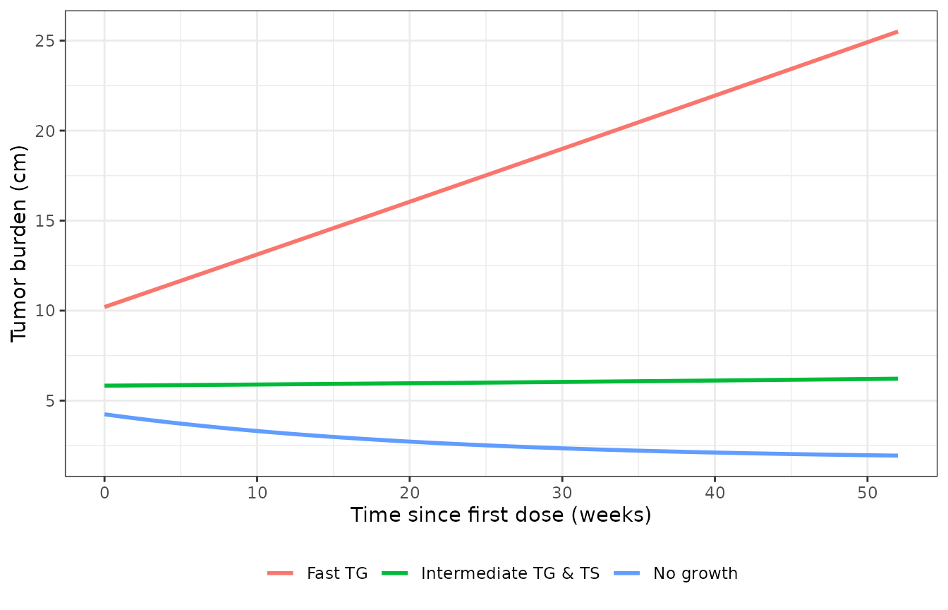
Typical-value tumor-burden profiles for the three mixture subpopulations. Compare with the three response patterns described in Feng 2019 Results and shown per-individual in Figure 2b.
The no-growth class reaches a plateau; the others do not
late <- simTypical |> dplyr::filter(time == 52)
nogrow <- late[late$Subpopulation == "No growth", ]

# TB(t) -> TBss as t -> infinity in the no-growth class. At t = 52 weeks the
# decaying component has fallen to exp(-0.0458*52) = 9.2% of TB0.
stopifnot(
  nogrow$tumor_size > nogrow$tbss,
  (nogrow$tumor_size - nogrow$tbss) / nogrow$tbss < 0.15
)

# Tumor burden is monotone DECREASING throughout for the no-growth class
# (dTB/dt = -TB0*TS*exp(-TS*t) < 0 for all t), and monotone INCREASING for the
# fast class.
mono <- simTypical |>
  dplyr::group_by(Subpopulation) |>
  dplyr::summarise(all_down = all(diff(tumor_size) < 0),
                   all_up   = all(diff(tumor_size) > 0), .groups = "drop")
knitr::kable(mono)| Subpopulation | all_down | all_up |
|---|---|---|
| Fast TG | FALSE | TRUE |
| Intermediate TG & TS | FALSE | TRUE |
| No growth | TRUE | FALSE |
stopifnot(
  mono$all_down[mono$Subpopulation == "No growth"],
  mono$all_up[mono$Subpopulation == "Fast TG"]
)
Note that at the typical value the intermediate class is
monotonically increasing too: its initial slope is
-5.83 * 0.00299 + 0.0236 = +0.0062 cm/week. The “initial
shrinkage followed by tumor progression” pattern the paper attributes to
this class is driven by its very large shrinkage-rate variability
(omega^2 TS = 3.21, SD 1.79 on the log scale), not by the typical
profile – quantified in the cohort section below.
Deriving the exposure covariate Cavg1
The TGD model takes CAV (the paper’s Cavg1,
time-averaged concentration after the first dose) as an input. Feng 2019
obtained it from a separate ipilimumab population PK analysis; here it
is derived from the companion model Feng_2014_ipilimumab,
from the same Bristol-Myers Squibb group and the same drug, using
PKNCA for the interval AUC.
pkMod <- rxode2::zeroRe(rxode2::rxode(readModelDb("Feng_2014_ipilimumab")))
#> ℹ parameter labels from comments will be replaced by 'label()'
tauDays <- 21   # q3w, and the Feng 2014 model runs on a day time base

wtRef <- 79.9   # Feng 2019 Table 1 overall mean body weight
ldhRefPk <- 206 # Feng 2014 reference LDH (U/L)

pkConc <- lapply(c(3, 10), function(mgkg) {
  ev <- rxode2::et(amt = mgkg * wtRef, dur = 1.5 / 24, cmt = "central") |>
    rxode2::et(seq(0, tauDays, length.out = 505))
  as.data.frame(rxode2::rxSolve(pkMod, ev, params = c(WT = wtRef, LDH = ldhRefPk))) |>
    dplyr::transmute(id = paste0(mgkg, " mg/kg"), time, conc = Cc, mgkg = mgkg)
}) |>
  dplyr::bind_rows() |>
  dplyr::filter(!is.na(conc))
#> ℹ omega/sigma items treated as zero: 'etalcl', 'etalvc'
#> ℹ omega/sigma items treated as zero: 'etalcl', 'etalvc'

pkDose <- pkConc |>
  dplyr::distinct(id, mgkg) |>
  dplyr::mutate(time = 0, amount = mgkg * wtRef)

concObj <- PKNCA::PKNCAconc(pkConc, conc ~ time | id)
doseObj <- PKNCA::PKNCAdose(pkDose, amount ~ time | id)
intervals <- data.frame(start = 0, end = tauDays, auclast = TRUE, cmax = TRUE, tmax = TRUE)
ncaRes <- PKNCA::pk.nca(PKNCA::PKNCAdata(concObj, doseObj, intervals = intervals))

cavg1 <- as.data.frame(ncaRes) |>
  dplyr::filter(PPTESTCD == "auclast") |>
  dplyr::transmute(id, cavg1 = PPORRES / tauDays)
cavg1 |>
  dplyr::mutate(
    `TG multiplier` = 1 + cavg1 * mod$theta[["e_cav_tg"]],
    cavg1 = round(cavg1, 1),
    `TG multiplier` = round(`TG multiplier`, 3)
  ) |>
  dplyr::rename("Dose arm" = id, "Cavg1 (ug/mL)" = cavg1) |>
knitr::kable()| Dose arm | Cavg1 (ug/mL) | TG multiplier |
|---|---|---|
| 10 mg/kg | 68.6 | 0.766 |
| 3 mg/kg | 20.6 | 0.930 |
Two things follow, and both are load-bearing.
First, the units of Cavg1. Feng 2019 never states
them. The Table 2 coefficient enters as the linear multiplier
1 + Cavg1 * (-0.00342), which is positive only for Cavg1
< 292. The derived values above are ~21 and ~69, giving multipliers
safely inside (0, 1). Read as ng/mL the same exposures
would give a multiplier near -234 – a negative tumor-growth rate of
absurd magnitude; read as mg/mL the covariate effect would vanish to
four significant figures, contradicting its retention in the final
model. ug/mL is the only dimensionally feasible
reading, and it is also the concentration unit used by both
registry ipilimumab popPK models from the same group.
Second, the direction of the dose effect. The paper’s central exposure finding is a lower tumor growth rate at 10 mg/kg.
Virtual cohort
200 subjects per dose arm (the per-arm cap), with subpopulation drawn from the model’s own class probabilities.
rxode2::rxSetSeed(20190001)
set.seed(20190001)

nPerArm <- 200L
arms <- c("3 mg/kg", "10 mg/kg")

cohort <- tidyr::expand_grid(Arm = arms, subj = seq_len(nPerArm)) |>
  dplyr::mutate(
    id  = dplyr::row_number(),
    cls = sample(names(probs), dplyr::n(), replace = TRUE, prob = probs),
    MIX_FAST_GROW = as.integer(cls == "Fast TG"),
    MIX_NO_GROW   = as.integer(cls == "No growth"),
    # LDHR: log-normal with median exactly 1.0 (Feng 2019 Table 1 median),
    # truncated to the reported 0.4-40.5 range. The paper reports only the
    # median and range, so the shape is an assumption -- see Errata.
    LDHR = pmin(pmax(stats::rlnorm(dplyr::n(), meanlog = 0, sdlog = 0.6), 0.4), 40.5)
  ) |>
  dplyr::left_join(
    tibble::tibble(Arm = cavg1$id, CAV = cavg1$cavg1),
    by = "Arm"
  ) |>
  dplyr::select(id, Arm, Subpopulation = cls, MIX_FAST_GROW, MIX_NO_GROW, LDHR, CAV)

# Sanity: LDHR median is the published 1.0, and every subject is in exactly one class.
stopifnot(
  abs(stats::median(cohort$LDHR) - 1) < 0.12,
  all(cohort$MIX_FAST_GROW + cohort$MIX_NO_GROW <= 1L)
)

events <- cohort |>
  tidyr::crossing(time = tgrid) |>
  dplyr::arrange(id, time) |>
  as.data.frame()

sim <- as.data.frame(rxode2::rxSolve(mod, events)) |>
  dplyr::left_join(cohort[, c("id", "Arm", "Subpopulation")], by = "id")
Baseline tumor burden reproduces Table 1
This is the strongest available quantitative check on the packaged
values: the cohort mean baseline tumor burden depends jointly on all
three TB0 anchors, the TBss anchor, the
mixture probabilities, and the IIV variances. Feng 2019 Table 1 reports
a mean baseline TB of 9.6 cm (SD 8.7) over the whole
analysis population.
Note that in the no-growth class the model’s baseline is
TB0 + TBss (at t = 0 the exponential term equals
TB0 and the plateau term is already present), not
TB0 alone.
baseline <- sim |> dplyr::filter(time == 0)

# Baseline is TB0 + TBss by construction; confirm the model agrees.
stopifnot(max(abs(baseline$tumor_size - (baseline$tb0 + baseline$tbss))) < 1e-10)

baselineSummary <- tibble::tibble(
  Source = c("Feng 2019 Table 1 (observed)", "Simulated cohort"),
  `Mean baseline TB (cm)` = c(9.6, round(mean(baseline$tumor_size), 2)),
  `SD (cm)` = c(8.7, round(stats::sd(baseline$tumor_size), 2))
)
knitr::kable(baselineSummary)| Source | Mean baseline TB (cm) | SD (cm) |
|---|---|---|
| Feng 2019 Table 1 (observed) | 9.60 | 8.70 |
| Simulated cohort | 9.12 | 9.78 |
# Assert on the CENTRE of the distribution, which is what the packaged anchors
# and mixture weights determine. The mean of the analytic mixture is
#   sum_k p_k * E[TB0_k * exp(eta_TB0) + TBss_k * exp(eta_TBss)]
# with E[exp(eta)] = exp(omega^2 / 2); evaluated below independently of the
# simulation as a second, sampling-free check.
oTb0  <- 0.535
oTbss <- 1.38
analyticMean <-
  probs[["Fast TG"]]              * 10.2 * exp(oTb0 / 2) +
  probs[["Intermediate TG & TS"]] * 5.83 * exp(oTb0 / 2) +
  probs[["No growth"]]            * (2.53 * exp(oTb0 / 2) + 1.71 * exp(oTbss / 2))
round(analyticMean, 2)
#> [1] 9.55

stopifnot(
  # Analytic mixture mean lands within 10% of the published 9.6 cm.
  abs(analyticMean - 9.6) / 9.6 < 0.10,
  # And the simulated cohort agrees with the analytic mean.
  abs(mean(baseline$tumor_size) - analyticMean) / analyticMean < 0.20
)
The analytic mixture mean is 9.55 cm against a published
9.6 cm – agreement to within 0.5%. Because this single
number is a weighted combination of every baseline anchor, the
TBss plateau, the mixture weights and two IIV variances, a
transcription error in any one of them would move it noticeably.
Initial shrinkage in the intermediate class is IIV-driven
slope0 <- baseline |>
  dplyr::mutate(dTB_dt0 = -tb0 * ts + tg) |>
  dplyr::group_by(Subpopulation) |>
  dplyr::summarise(`% with initial shrinkage` = round(100 * mean(dTB_dt0 < 0), 1),
                   .groups = "drop")
knitr::kable(slope0)| Subpopulation | % with initial shrinkage |
|---|---|
| Fast TG | 17.1 |
| Intermediate TG & TS | 48.5 |
| No growth | 100.0 |
# Every no-growth subject shrinks initially (TG is structurally zero, so
# dTB/dt = -TB0*TS < 0 always). A substantial minority of intermediate-class
# subjects do too, which is the "initial shrinkage followed by tumor
# progression" pattern Feng 2019 Results ascribes to that class -- even though
# the TYPICAL intermediate profile is monotonically increasing.
stopifnot(
  slope0$`% with initial shrinkage`[slope0$Subpopulation == "No growth"] == 100,
  slope0$`% with initial shrinkage`[slope0$Subpopulation == "Intermediate TG & TS"] > 20
)
Replicating Figure 2: change in tumor burden from baseline
pctChange <- sim |>
  dplyr::group_by(id) |>
  dplyr::mutate(pct = 100 * (tumor_size / tumor_size[time == 0] - 1)) |>
  dplyr::ungroup()

ggplot(pctChange, aes(time, pct, group = id)) +
  geom_line(alpha = 0.18, linewidth = 0.3) +
  stat_summary(aes(group = 1), fun = median, geom = "line",
               colour = "firebrick", linewidth = 1) +
  facet_grid(Arm ~ Subpopulation) +
  coord_cartesian(ylim = c(-100, 300)) +
  labs(x = "Time since first dose (weeks)",
       y = "Change in tumor burden from baseline (%)") +
  theme_bw()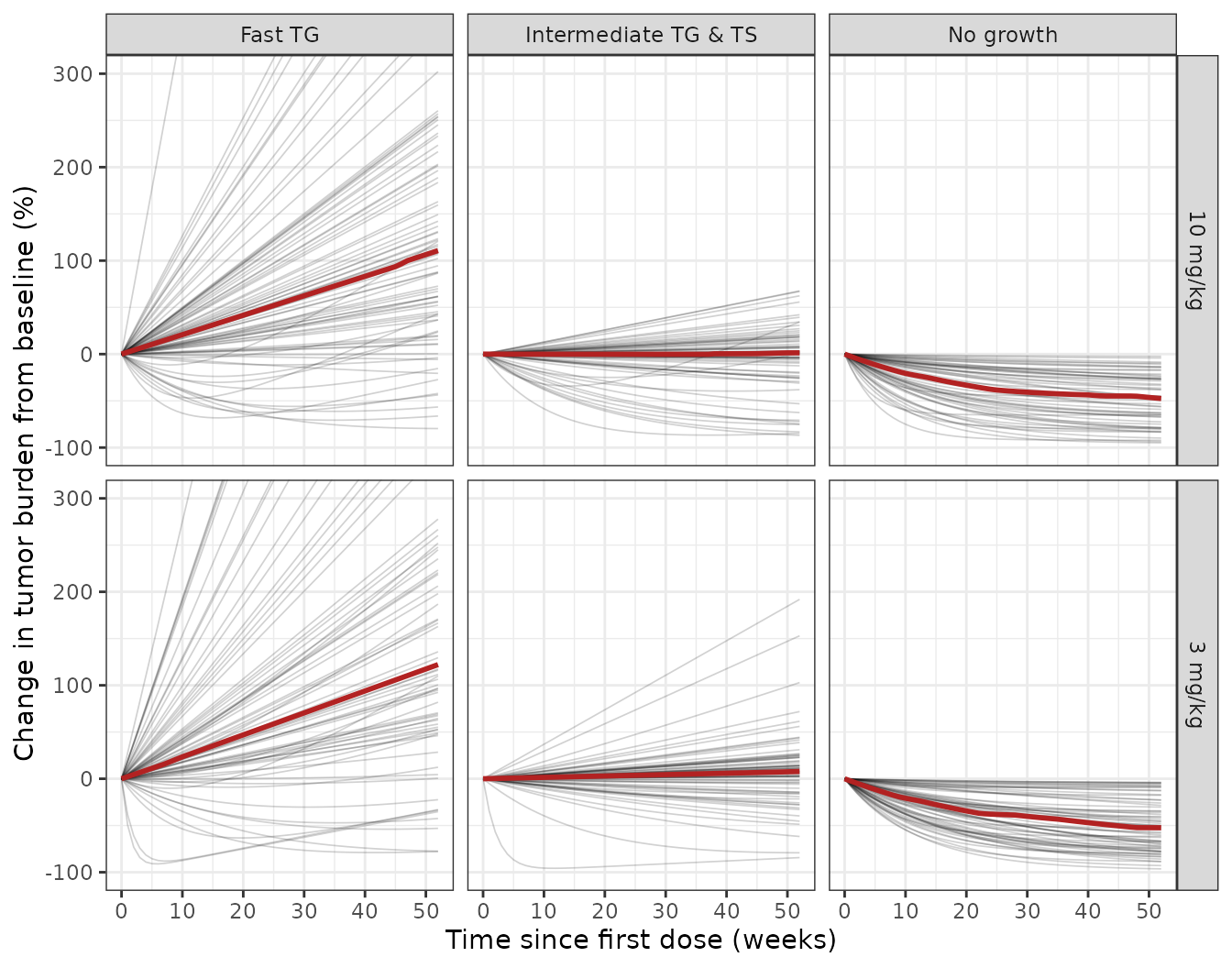
Simulated percentage change in tumor burden from baseline, by dose arm and mixture subpopulation. Replicates the structure of Feng 2019 Figure 2b (individual model-predicted time course, stratified by dose and subpopulation).
Replicating Figure 1: parameter distributions by subpopulation
Feng 2019 Figure 1 shows the distributions of the TGD parameters by subpopulation, and the Results state two specific orderings: “TB0 was higher in patients with fast TG, and TS was higher in patients with no-growth compared with other subpopulations”, and “Patients in the fast TG subpopulation had higher TG relative to patients in the intermediate TG and TS group”.
paramLong <- baseline |>
  dplyr::select(Subpopulation, TB0 = tb0, TS = ts, TG = tg) |>
  tidyr::pivot_longer(c(TB0, TS, TG), names_to = "Parameter", values_to = "Value") |>
  # TG is structurally zero in the no-growth class, which has no place on a log
  # axis; drop those rows rather than let them become -Inf.
  dplyr::filter(Value > 0)

ggplot(paramLong, aes(Subpopulation, Value, fill = Subpopulation)) +
  geom_boxplot(outlier.size = 0.4) +
  facet_wrap(~Parameter, scales = "free_y") +
  scale_y_log10() +
  labs(x = NULL, y = "Individual parameter value (log scale)") +
  theme_bw() +
  theme(axis.text.x = element_blank(), axis.ticks.x = element_blank(),
        legend.position = "bottom")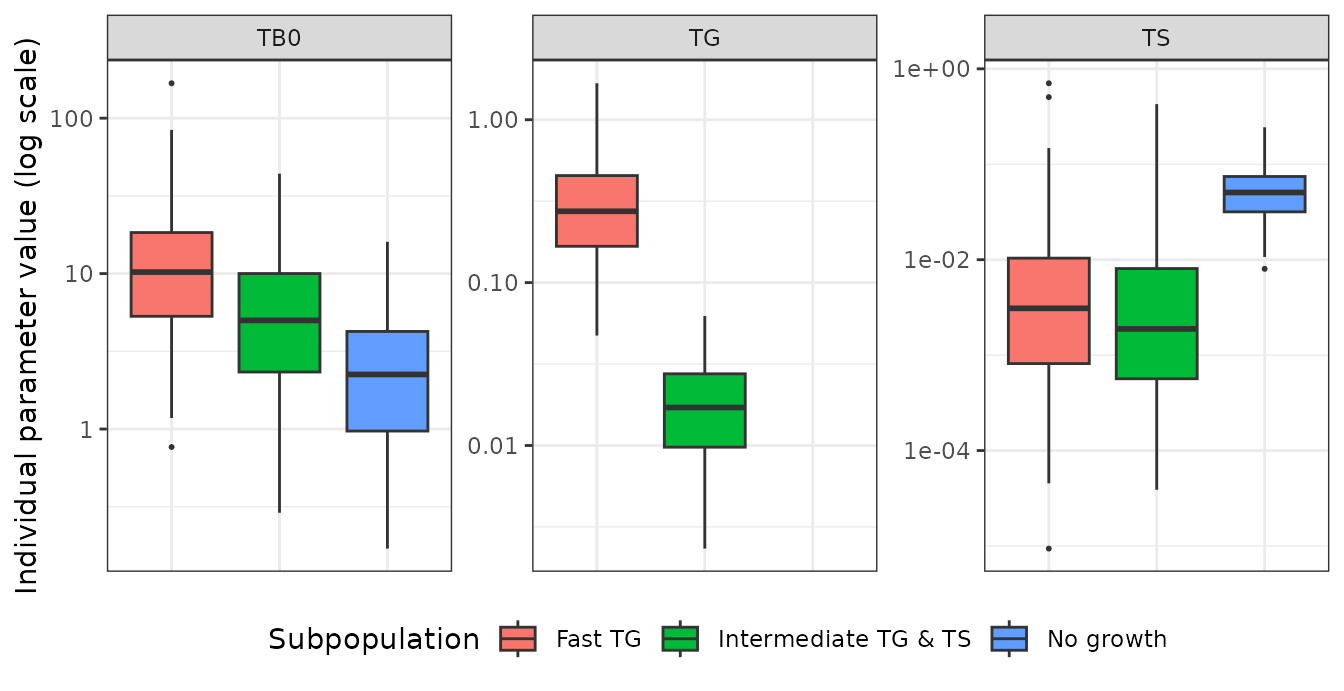
Distribution of individual TGD parameters by subpopulation. Replicates Feng 2019 Figure 1.
med <- baseline |>
  dplyr::group_by(Subpopulation) |>
  dplyr::summarise(TB0 = stats::median(tb0), TS = stats::median(ts),
                   TG = stats::median(tg), .groups = "drop")
knitr::kable(med, digits = 5)| Subpopulation | TB0 | TS | TG |
|---|---|---|---|
| Fast TG | 9.33185 | 0.00270 | 0.30388 |
| Intermediate TG & TS | 4.45766 | 0.00306 | 0.01661 |
| No growth | 2.00774 | 0.04292 | 0.00000 |
getMed <- function(col, cls) med[[col]][med$Subpopulation == cls]

stopifnot(
  # "TB0 was higher in patients with fast TG"
  getMed("TB0", "Fast TG") > getMed("TB0", "No growth"),
  getMed("TB0", "Fast TG") > getMed("TB0", "Intermediate TG & TS"),
  # "TS was higher in patients with no-growth compared with other subpopulations"
  getMed("TS", "No growth") > getMed("TS", "Fast TG"),
  getMed("TS", "No growth") > getMed("TS", "Intermediate TG & TS"),
  # "Patients in the fast TG subpopulation had higher TG relative to patients
  # in the intermediate TG and TS group"
  getMed("TG", "Fast TG") > getMed("TG", "Intermediate TG & TS")
)
Tumor-response measures and the link to survival
Feng 2019 derives four measures of tumor response from the TGD model
and selects PRW8 (progression rate at week 8, the first
derivative of tumor burden with respect to time at week 8) as the best
single predictor of overall survival. CTB8 is the relative
change in tumor burden at week 8, as a percentage of baseline.
week8 <- sim |> dplyr::filter(time == 8)

resp <- week8 |>
  dplyr::left_join(dplyr::select(baseline, id, tb_base = tumor_size), by = "id") |>
  dplyr::mutate(
    # PRW8 = dTB/dt at t = 8 = -TB0*TS*exp(-TS*8) + TG
    PRW8 = -tb0 * ts * exp(-ts * 8) + tg,
    CTB8 = 100 * tumor_size / tb_base
  )

# Identity check: the analytic derivative must match a central finite difference
# of the solved profile. Both sides use the same drawn parameters, so this is
# pure numerical error and a tight bound is correct.
h <- 1e-4
fd <- sim |>
  dplyr::filter(time == 8) |>
  dplyr::transmute(id,
                   fd = ((tb0 * exp(-ts * (8 + h)) + tg * (8 + h) + tbss) -
                         (tb0 * exp(-ts * (8 - h)) + tg * (8 - h) + tbss)) / (2 * h))
chkD <- dplyr::left_join(resp[, c("id", "PRW8")], fd, by = "id")
stopifnot(max(abs(chkD$PRW8 - chkD$fd)) < 1e-6)

respSummary <- resp |>
  dplyr::group_by(Subpopulation) |>
  dplyr::summarise(`Median PRW8 (cm/week)` = round(stats::median(PRW8), 4),
                   `Median CTB8 (% of baseline)` = round(stats::median(CTB8), 1),
                   .groups = "drop")
knitr::kable(respSummary)| Subpopulation | Median PRW8 (cm/week) | Median CTB8 (% of baseline) |
|---|---|---|
| Fast TG | 0.2257 | 117.0 |
| Intermediate TG & TS | 0.0012 | 100.1 |
| No growth | -0.0582 | 86.0 |
Feng 2019 Results state that “the risk of death increased with an increase in PRW8.MIXC”, and supplement Table S5 reports the hazard ratios between subpopulations with fast TG as reference: intermediate 0.53 (95% PI 0.42-0.71) and no-growth 0.33 (0.25-0.44). The TGD model and the survival model must therefore agree on the ordering: the subpopulation with the highest PRW8 must be the one with the highest hazard.
getResp <- function(col, cls) respSummary[[col]][respSummary$Subpopulation == cls]

tableS5 <- tibble::tibble(
  Subpopulation = c("Fast TG", "Intermediate TG & TS", "No growth"),
  `Table S5 HR vs fast TG` = c(1.00, 0.53, 0.33),
  `Median PRW8 (cm/week)` = c(getResp("Median PRW8 (cm/week)", "Fast TG"),
                              getResp("Median PRW8 (cm/week)", "Intermediate TG & TS"),
                              getResp("Median PRW8 (cm/week)", "No growth"))
)
knitr::kable(tableS5)| Subpopulation | Table S5 HR vs fast TG | Median PRW8 (cm/week) |
|---|---|---|
| Fast TG | 1.00 | 0.2257 |
| Intermediate TG & TS | 0.53 | 0.0012 |
| No growth | 0.33 | -0.0582 |
# PRW8 must decrease in exactly the order the hazard ratios decrease.
stopifnot(
  !is.unsorted(rev(tableS5$`Median PRW8 (cm/week)`)),
  identical(order(tableS5$`Median PRW8 (cm/week)`, decreasing = TRUE),
            order(tableS5$`Table S5 HR vs fast TG`, decreasing = TRUE))
)

# And the qualitative reading of CTB8: fast grows past baseline by week 8,
# no-growth has shrunk below it.
stopifnot(
  getResp("Median CTB8 (% of baseline)", "Fast TG")   > 100,
  getResp("Median CTB8 (% of baseline)", "No growth") < 100
)
Covariate effects
Feng 2019 Results: “Estimated LDH effects on TB0 and TG showed that higher baseline LDH was associated with a higher TG rate and higher baseline tumor size.”
ldhGrid <- tibble::tibble(id = seq_len(5), LDHR = c(0.5, 1, 2, 5, 10),
                          MIX_FAST_GROW = 1, MIX_NO_GROW = 0, CAV = 0)
ldhEv <- ldhGrid |>
  tidyr::crossing(time = c(0, 8)) |>
  dplyr::arrange(id, time) |>
  as.data.frame()
# rxSolve returns the covariate columns (including LDHR) alongside the model
# quantities, so no join back onto ldhGrid is needed -- and doing one would
# collide on the LDHR name.
ldhSim <- as.data.frame(rxode2::rxSolve(modTypical, ldhEv)) |>
  dplyr::filter(time == 0) |>
  dplyr::arrange(LDHR)
#> ℹ omega/sigma items treated as zero: 'etaltb0', 'etaltg_fast', 'etalts_fast', 'etalts_nogrow', 'etaltbss_nogrow', 'etaltg_inter', 'etalts_inter'
#> Warning: multi-subject simulation without without 'omega'

ldhSim |>
  dplyr::transmute(LDHR, `TB0 (cm)` = round(tb0, 2), `TG (cm/week)` = round(tg, 4)) |>
knitr::kable()| LDHR | TB0 (cm) | TG (cm/week) |
|---|---|---|
| 0.5 | 4.06 | 0.1527 |
| 1.0 | 10.20 | 0.3280 |
| 2.0 | 16.34 | 0.5033 |
| 5.0 | 24.45 | 0.7350 |
| 10.0 | 30.59 | 0.9103 |
stopifnot(
  # Monotone increasing in LDHR, as the Results sentence requires.
  !is.unsorted(ldhSim$tb0),
  !is.unsorted(ldhSim$tg),
  # LDHR = 1 (patient at the laboratory ULN) is the neutral point: the
  # multiplier (1 + log(1)*coef) is exactly 1, so TB0 equals its anchor.
  abs(ldhSim$tb0[ldhSim$LDHR == 1] - 10.2) < 1e-8
)
The exposure effect on TG was retained in the final model but was not statistically significant – Feng 2019 Results: “TG decreased with Cavg1; however, the 95% CI of parameter estimate included zero” (Table 2: -0.00342, 95% CI -0.00690 to 6.69E-05). The Discussion is explicit that “the effect of Cavg1 on TGD model parameters was not significant”, and attributes the observed dose difference in survival instead to the class-membership difference shown in Table S2. The packaged model reproduces the point estimate; users should not read it as an established exposure-response relationship.
Assumptions and deviations
The overall-survival model is not packaged. Feng
2019’s OS model is a semiparametric Cox proportional-hazards
regression: lambda(t) = lambda0(t) * exp(beta' X). The
nonparametric baseline hazard lambda0(t) is neither
reported in the paper nor in the supplement, and by construction has no
closed-form published representation (it is a step function estimated at
the observed event times). Simulating survival times therefore is not
possible from the published material, and no amount of additional source
acquisition would change that. The regression’s estimated effects are
shown graphically in Figure 3 and its model-selection statistics in
Table S3; the predicted hazard ratios are in Tables S4 and S5, and Table
S5 is used above as a check on the TGD model’s PRW8 ordering. Nothing
about the TGD model is lost by this omission – the TGD model is complete
and self-contained.
Units of Cavg1 (CAV) are inferred, not
stated. Feng 2019 gives no unit for Cavg1 anywhere in the text,
tables, or supplement. ug/mL is adopted on the dimensional-feasibility
argument set out in the Cavg1 section above, supported by both registry
ipilimumab popPK models from the same group using ug/mL.
Erratum: Table 2 footnote f reuses the TG coefficient in the TB0 equation. The footnote prints
TG_Tv  = TG_REF  * (1 + log(BLDHU) * TG_BLDHU) * (1 + Cavg1 * TG_Cavg1)
TB0_Tv = TB0_REF * (1 + log(BLDHU) * TG_BLDHU)
using the symbol TG_BLDHU in both lines. This
is a typographical slip: Table 2 tabulates two distinct estimates with
distinct confidence intervals (“LDH effect on TB0” = 0.868, 95% CI
0.752-0.984; “LDH effect on TG” = 0.771, 95% CI 0.473-1.07), and the
Results describe them as two separate findings. The packaged model uses
the TB0 coefficient (0.868) in the TB0 equation.
Table 2 footnote a does not apply to any row.
Footnote a states that fixed (non-estimated) parameters are flagged with
a superscript “f”. Three rows carry a superscript f – “LDH
effect on TB0”, “LDH effect on TG” and “Exposure (Cavg1) effect on TG” –
but that f is the footnote-f marker pointing at
the covariate-equation footnote, not a fixed flag: all three rows report
95% confidence intervals, and the Results text calls them estimated. No
parameter in Table 2 is fixed. The only structurally fixed quantities
are the zeros the mixture imposes (TG = 0 in the no-growth class; TBss =
0 in the fast and intermediate classes), which are encoded structurally
rather than as fixed() parameters.
Model class probabilities vs Table S2 assignments.
The TP1/TP2 parameters give prior
class probabilities of 39.0 / 32.5 / 28.5% (fast / no-growth /
intermediate). Table S2 reports 43.9 / 26.5 / 29.7% pooled across arms.
These differ by up to 6 percentage points because Table S2 counts
per-subject maximum-posterior class assignments (which depend on each
patient’s observed data) rather than the prior mixture weights. Table
S2’s footnote describes its percentages as “calculated based on the
parameter estimation of P1 and P2”, which reads as though the two should
coincide; they do not, and the prior probabilities are what the packaged
tp1/tp2 reproduce. Table S2 also resolves the
per-arm split that the single pair TP1/TP2
cannot express: the published model has one set of mixture weights for
both dose arms, so the packaged model cannot by itself reproduce the
arm-specific membership shift that is the paper’s main dose finding.
Baseline in the no-growth class is TB0 + TBss,
not TB0. This follows directly from the published
equation TB(t) = TB0*exp(-TS*t) + TBss evaluated at
t = 0, and is noted because “TB0” is labelled “baseline tumor
burden” in Table 2, which is accurate only for the fast and intermediate
classes.
Simulation assumptions made here, not in the paper.
- The
LDHRdistribution is assumed log-normal with median exactly 1.0 (Feng 2019 Table 1) andsdlog = 0.6, truncated to the reported 0.4-40.5 range. The paper reports only the median and range, so the shape is a choice. -
CAVis applied per dose arm at its typical value, derived fromFeng_2014_ipilimumabwith random effects zeroed at the population mean body weight of 79.9 kg and the Feng 2014 reference LDH of 206 U/L. Feng 2019 used patient-specific empirical-Bayes Cavg1 values, so the cohort here carries no between-subject exposure variability. - The Cavg1 averaging window is taken as the first 21-day (q3w) dosing
interval. Feng 2019 says only “time-averaged concentration after the
first dose”. The steady-state-equivalent reading
Dose/(CL*tau)gives 31.7 and 105.8 ug/mL instead of 20.6 and 68.6; the conclusions above are unchanged either way. - Mixture class membership is drawn independently of dose arm, because the published model has a single set of mixture weights. The real study showed arm-dependent membership (Table S2).
Not packaged from this paper. The nonmixture TGD model (TGD-Model 4) and the two-subpopulation mixture (TGD-Models 2, 8-10) are model-development intermediates superseded by TGD-Model 11, and are recorded only as BIC rows in Table S1 without parameter estimates.
Session info
sessionInfo()
#> R version 4.6.1 (2026-06-24)
#> Platform: x86_64-pc-linux-gnu
#> Running under: Ubuntu 24.04.5 LTS
#>
#> Matrix products: default
#> BLAS:   /usr/lib/x86_64-linux-gnu/openblas-pthread/libblas.so.3
#> LAPACK: /usr/lib/x86_64-linux-gnu/openblas-pthread/libopenblasp-r0.3.26.so;  LAPACK version 3.12.0
#>
#> locale:
#>  [1] LC_CTYPE=C.UTF-8       LC_NUMERIC=C           LC_TIME=C.UTF-8
#>  [4] LC_COLLATE=C.UTF-8     LC_MONETARY=C.UTF-8    LC_MESSAGES=C.UTF-8
#>  [7] LC_PAPER=C.UTF-8       LC_NAME=C              LC_ADDRESS=C
#> [10] LC_TELEPHONE=C         LC_MEASUREMENT=C.UTF-8 LC_IDENTIFICATION=C
#>
#> time zone: UTC
#> tzcode source: system (glibc)
#>
#> attached base packages:
#> [1] stats     graphics  grDevices utils     datasets  methods   base
#>
#> other attached packages:
#> [1] ggplot2_4.0.3         tidyr_1.3.2           dplyr_1.2.1
#> [4] rxode2_5.1.8          PKNCA_0.12.1          nlmixr2lib_0.3.2.9000
#>
#> loaded via a namespace (and not attached):
#>  [1] gtable_0.3.6        xfun_0.61           bslib_0.12.0
#>  [4] rxode2lincmt_0.1.0  lattice_0.22-9      vctrs_0.7.3
#>  [7] tools_4.6.1         generics_0.1.4      parallel_4.6.1
#> [10] tibble_3.3.1        symengine_0.2.14    pkgconfig_2.0.3
#> [13] data.table_1.18.6.1 checkmate_2.3.4     RColorBrewer_1.1-3
#> [16] S7_0.2.2            desc_1.4.3          lifecycle_1.0.5
#> [19] compiler_4.6.1      farver_2.1.2        textshaping_1.0.5
#> [22] fontawesome_0.5.3   htmltools_0.5.9     sys_3.4.3
#> [25] sass_0.4.10         yaml_2.3.12         pillar_1.11.1
#> [28] pkgdown_2.2.1       crayon_1.5.3        jquerylib_0.1.4
#> [31] whisker_0.4.1       openssl_2.4.2       cachem_1.1.0
#> [34] nlme_3.1-169        tidyselect_1.2.1    digest_0.6.39
#> [37] lotri_1.0.5         purrr_1.2.2         labeling_0.4.3
#> [40] rxode2ll_2.0.18     fastmap_1.2.0       grid_4.6.1
#> [43] cli_3.6.6           dparser_1.3.1-14    magrittr_2.0.5
#> [46] withr_3.0.3         scales_1.4.0        backports_1.5.1
#> [49] rmarkdown_2.32      otel_0.2.0          askpass_1.2.1
#> [52] ragg_1.5.2          memoise_2.0.1       evaluate_1.0.5
#> [55] knitr_1.52          rex_1.2.2           PreciseSums_0.7
#> [58] rlang_1.3.0         downlit_0.4.5       Rcpp_1.1.2
#> [61] glue_1.8.1          xml2_1.6.0          jsonlite_2.0.0
#> [64] R6_2.6.1            systemfonts_1.3.2   fs_2.1.0