Model and source
- Citation: Dong Q, Chen C, Taubert M, Bilal M, Kinzig M, Sorgel F, Scherf-Clavel O, Fuhr U, Dokos C. Understanding adefovir pharmacokinetics as a component of a transporter phenotyping cocktail. Eur J Clin Pharmacol. 2024;80(7):1069-1078. doi:10.1007/s00228-024-03673-x
- Description: One-compartment population PK model for adefovir after a single oral 10 mg dose of the prodrug adefovir dipivoxil in healthy adults, given alone (reference period) and together with the four other components of a transporter phenotyping cocktail (metformin, sitagliptin, pitavastatin and digoxin; test period) (Dong 2024). First-order absorption with a lag time; elimination is the sum of a linear nonrenal clearance and a Michaelis-Menten renal arm that feeds a urinary-excretion compartment, with Vmax proportional to the absolute estimated GFR. The cocktail raises the apparent bioavailability and lowers the absorption rate constant. Inter-individual variability on V and Vmax; inter-occasion variability (two periods) on F, ka, lag time and V; proportional residual error on plasma concentration and on urinary amount.
- Article: https://doi.org/10.1007/s00228-024-03673-x (open access, PMC11156719)
Adefovir dipivoxil is the renal OAT1 probe of a five-drug transporter phenotyping cocktail (adefovir dipivoxil, metformin, sitagliptin, pitavastatin and digoxin). In the cocktail trial adefovir exposure was about 20% higher with the other four drugs than alone. Dong 2024 refit the plasma and urine data with a population model to locate the interaction: it sits in the apparent absorption (higher F, slower ka), not in the saturable renal elimination.
Population
Twenty-four healthy adults (10 male, 14 female) from the Cologne cocktail phenotyping trial (NCT02743260): median age 35 years (range 20-68), body weight 71.3 kg (55.5-94.9), BMI 24.5 kg/m^2 (19.5-29.7) and absolute estimated GFR (CKD-EPI 2012 creatinine-cystatin C equation, de-normalised to the Mosteller body surface area) 105 mL/min (77.5-136) (Dong 2024 Supplemental Table 1s). Each subject received a single oral 10 mg dose of adefovir dipivoxil in a reference period (alone) and in a test period (with metformin, sitagliptin, pitavastatin and digoxin). Plasma was sampled and urine collected (0-4, 4-8, 8-12, 12-16 and 16-24 h) up to 24 h; 1101 plasma and urine values entered the analysis.
The same information is available programmatically via
readModelDb("Dong_2024_adefovir")()$population.
Source trace
Every value is also traced by an in-file comment in
inst/modeldb/specificDrugs/Dong_2024_adefovir.R.
| Equation / parameter | Value | Source location |
|---|---|---|
| Structure: depot -> central -> (nonrenal elimination, Michaelis-Menten renal arm -> urine) | – | Table 1, ‘Model 2’; Results ‘Adefovir base model’ |
fu = 1 (MM term on total concentration) |
– | Methods ‘Basic population pharmacokinetic analysis’ |
ltlag |
log(0.122 h) | Table 3, ALAG |
lvc |
log(235 L) | Table 3, V |
lcl_nonren |
log(11.8 L/h) | Table 3, CLNR |
lkm |
log(0.170 umol/L) | Table 3, Km = 170 nmol/L |
lvmax |
log(2.40 umol/h) | Table 3, Vmax |
vmax * (CRCL / 105) |
– | Results ‘Final model with demographic and physiological covariates’ (TVVmax equation) |
lfdepot |
fixed(log(0.590)) | Table 3, FR (fixed to the published value) |
lka |
log(5.18 1/h) | Table 3, KaR |
e_conmed_..._fdepot |
log(0.736 / 0.590) | Table 3, FT vs FR |
e_conmed_..._ka |
log(2.29 / 5.18) | Table 3, KaT vs KaR |
etalvc, etalvmax
|
0.028822, 0.035831 | Table 3 IIV 17.1%, 19.1% CV; omega^2 = log(CV^2 + 1) (Table 3 footnote) |
etaiov_fdepot_*, etaiov_ka_*,
etaiov_tlag_*, etaiov_vc_*
|
0.078095, 0.73314, 0.46459, 0.0068654 | Table 3 IOV 28.5%, 104%, 76.9%, 8.30% CV |
propSd |
0.094787 | Table 3 plasma 9.50% CV; sigma = sqrt(log(CV^2 + 1)) |
propSd_Aurine |
0.27568 | Table 3 urine 28.1% CV |
Virtual cohort
A crossover cohort of 200 subjects: each receives 10 mg adefovir dipivoxil (19.94 umol adefovir equivalents) alone at time 0 (occasion 1) and with the cocktail one week later (occasion 2), so the inter-occasion etas and the cocktail indicator change between periods exactly as in the trial. Absolute eGFR is drawn log-normally around the cohort median and truncated to the observed range.
mod <- readModelDb("Dong_2024_adefovir")

dose_umol <- 10 / 501.47 * 1000 # 10 mg adefovir dipivoxil, MW 501.47 g/mol
period_start <- c(reference = 0, test = 168)
obs_rel <- sort(unique(c(
  0, 0.25, 0.5, 0.75, 1, 1.25, 1.5, 2, 2.5, 3, 4, 5, 6, 8, 10, 12, 16, 20, 24
)))
n_sub <- 200

set.seed(20240607)
cohort <- tibble(
  id = seq_len(n_sub),
  CRCL = pmin(pmax(exp(rnorm(n_sub, log(105), 0.15)), 77.5), 136)
)

period_rows <- function(period, start) {
  occ <- if (period == "reference") 1 else 2
  conmed <- if (period == "reference") 0 else 1
  dose <- tibble(time = start, evid = 1L, amt = dose_umol, cmt = "depot", dvid = NA_integer_)
  # Observations sit on the ODE state; dvid = 1 maps them to the first
  # endpoint, and rxode2 returns both Cc and Aurine on every record.
  obs <- tibble(time = start + obs_rel, evid = 0L, amt = NA_real_, cmt = "central", dvid = 1L)
  bind_rows(dose, obs) |>
    mutate(
      period = period,
      OCC = occ,
      CONMED_DIGOXIN_METFORMIN_PITAVASTATIN_SITAGLIPTIN = conmed
    )
}

ev_template <- bind_rows(
  period_rows("reference", period_start[["reference"]]),
  period_rows("test", period_start[["test"]])
)

events <- cohort |>
  tidyr::crossing(ev_template) |>
  arrange(id, time, desc(evid)) |>
  as.data.frame()
Simulation
rxode2::rxSetSeed(20240607)
sim <- rxode2::rxSolve(
  mod,
  events = events,
  keep = c("period", "CRCL"),
  returnType = "data.frame"
)
#> ℹ parameter labels from comments will be replaced by 'label()'
#> Warning: some etas defaulted to non-mu referenced, possible parsing error: etaiov_fdepot_1, etaiov_fdepot_2, etaiov_ka_1, etaiov_ka_2, etaiov_tlag_1, etaiov_tlag_2, etaiov_vc_1, etaiov_vc_2
#> as a work-around try putting the mu-referenced expression on a simple line

sim <- sim |>
  mutate(
    period = factor(period, levels = c("reference", "test")),
    tad = time - period_start[as.character(period)]
  )

# Urinary amount per collection interval: difference of the cumulative
# urine state across the 0-4, 4-8, 8-12, 12-16 and 16-24 h boundaries.
urine_bounds <- c(0, 4, 8, 12, 16, 24)
urine_int <- sim |>
  filter(tad %in% urine_bounds) |>
  group_by(id, period) |>
  arrange(tad, .by_group = TRUE) |>
  mutate(
    ae_interval = urine - lag(urine),
    interval = paste0(lag(tad), "-", tad)
  ) |>
  filter(!is.na(ae_interval)) |>
  ungroup()
Typical-value profiles (no random effects) for the two periods:
mod_typ <- rxode2::zeroRe(mod)
#> ℹ parameter labels from comments will be replaced by 'label()'
#> Warning: some etas defaulted to non-mu referenced, possible parsing error: etaiov_fdepot_1, etaiov_fdepot_2, etaiov_ka_1, etaiov_ka_2, etaiov_tlag_1, etaiov_tlag_2, etaiov_vc_1, etaiov_vc_2
#> as a work-around try putting the mu-referenced expression on a simple line
#> Warning: some etas defaulted to non-mu referenced, possible parsing error: etaiov_fdepot_1, etaiov_fdepot_2, etaiov_ka_1, etaiov_ka_2, etaiov_tlag_1, etaiov_tlag_2, etaiov_vc_1, etaiov_vc_2
#> as a work-around try putting the mu-referenced expression on a simple line
typ_events <- events |> filter(id == 1) |> mutate(CRCL = 105)
typ <- rxode2::rxSolve(mod_typ, events = typ_events, keep = "period", returnType = "data.frame") |>
  mutate(tad = time - period_start[period])
#> ℹ omega/sigma items treated as zero: 'etalvc', 'etalvmax', 'etaiov_fdepot_1', 'etaiov_fdepot_2', 'etaiov_ka_1', 'etaiov_ka_2', 'etaiov_tlag_1', 'etaiov_tlag_2', 'etaiov_vc_1', 'etaiov_vc_2'

ggplot(typ, aes(tad, Cc, colour = period)) +
  geom_line() +
  labs(
    x = "Time after dose (h)", y = "Adefovir plasma concentration (nmol/L)",
    colour = "Period", title = "Typical subject (AGFR 105 mL/min)"
  ) +
  theme_bw()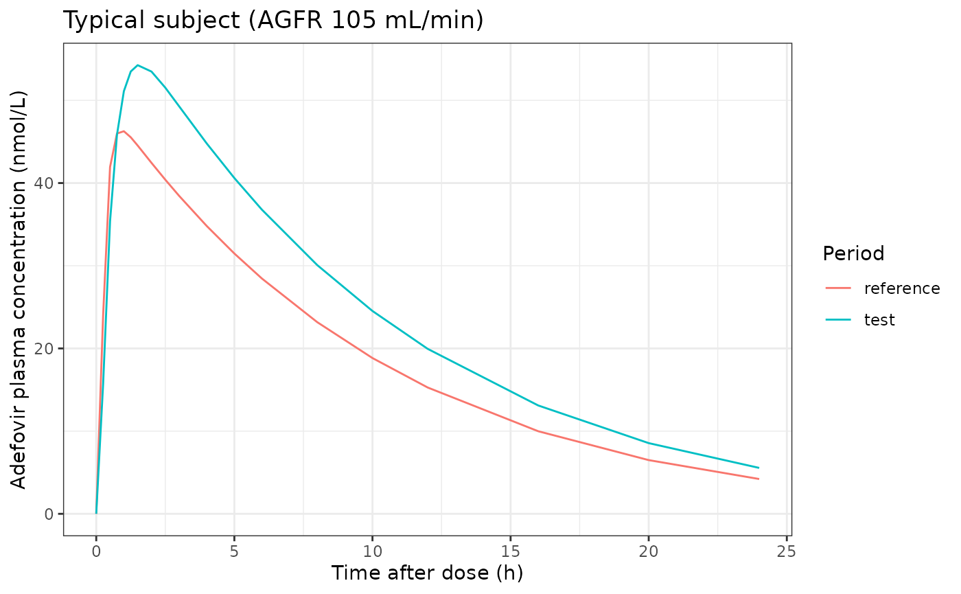
Replicate Figure 1 (VPC, nonlinear model)
Figure 1 pools both periods. The bands below are the simulated 2.5th, 50th and 97.5th percentiles; the black points are the observed medians read approximately from the Figure 1 urine panel (digitised by the maintainers).
vpc_plasma <- sim |>
  group_by(tad) |>
  summarise(
    p025 = quantile(Cc, 0.025),
    p50 = median(Cc),
    p975 = quantile(Cc, 0.975),
    .groups = "drop"
  )
ggplot(vpc_plasma, aes(tad)) +
  geom_ribbon(aes(ymin = p025, ymax = p975), fill = "lightblue") +
  geom_line(aes(y = p50), colour = "blue") +
  labs(x = "Time after last dose (h)", y = "Plasma adefovir (nmol/L)") +
  theme_bw()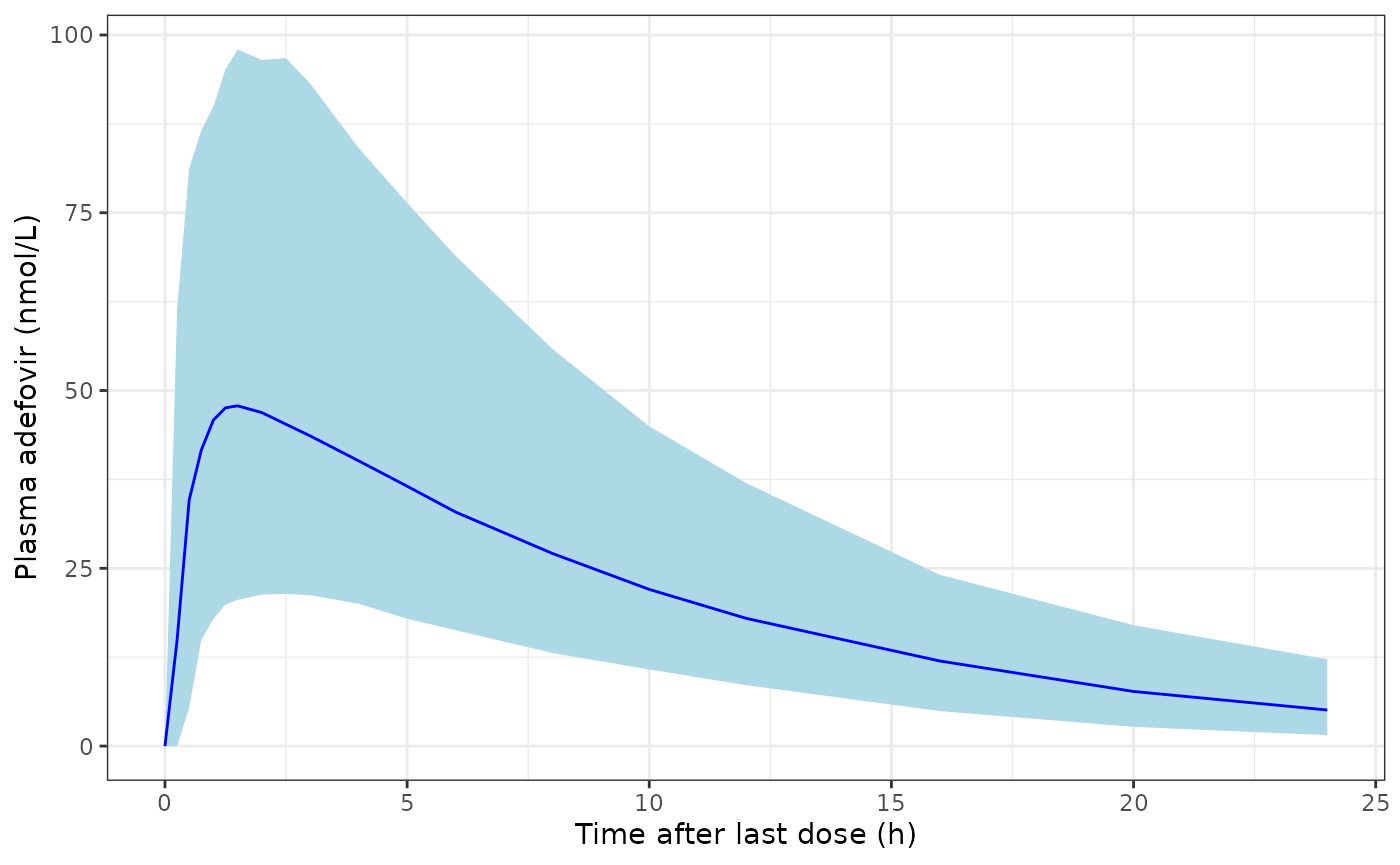
Replicates Figure 1 (right column, plasma) of Dong 2024: simulated plasma adefovir percentiles.
fig1_urine_obs <- tibble(
  tad = c(4, 8, 12, 16, 24),
  obs_median = c(2.0, 1.75, 1.2, 0.75, 0.8) # umol, approximate, Figure 1
)
vpc_urine <- urine_int |>
  group_by(tad) |>
  summarise(
    p025 = quantile(ae_interval, 0.025),
    p50 = median(ae_interval),
    p975 = quantile(ae_interval, 0.975),
    .groups = "drop"
  ) |>
  left_join(fig1_urine_obs, by = "tad")
ggplot(vpc_urine, aes(tad)) +
  geom_ribbon(aes(ymin = p025, ymax = p975), fill = "lightblue") +
  geom_line(aes(y = p50), colour = "blue") +
  geom_point(aes(y = obs_median)) +
  labs(x = "Time after last dose (h)", y = "Urinary adefovir per interval (umol)") +
  theme_bw()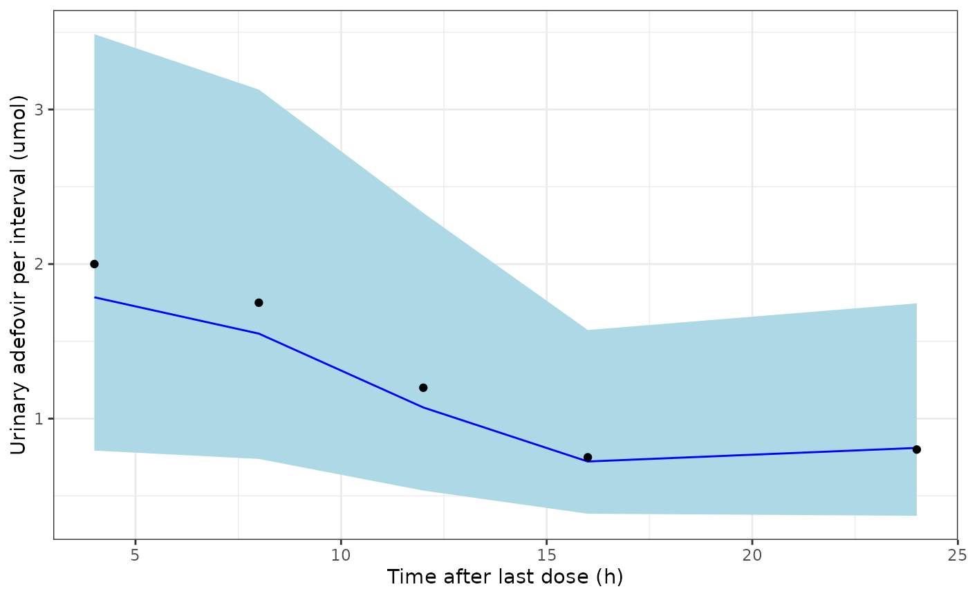
Replicates Figure 1 (right column, urine) of Dong 2024: simulated urinary amount per collection interval, plotted at the interval end.
knitr::kable(vpc_urine, digits = 2, caption = "Simulated percentiles vs approximate observed medians (Figure 1).")| tad | p025 | p50 | p975 | obs_median |
|---|---|---|---|---|
| 4 | 0.79 | 1.79 | 3.49 | 2.00 |
| 8 | 0.74 | 1.55 | 3.13 | 1.75 |
| 12 | 0.53 | 1.07 | 2.33 | 1.20 |
| 16 | 0.38 | 0.72 | 1.57 | 0.75 |
| 24 | 0.37 | 0.81 | 1.75 | 0.80 |
PKNCA validation
PKNCA runs on the plasma profile of each subject and period. The dose is passed in nmol so that clearance and volume come out in L/h and L.
conc_df <- sim |>
  filter(!is.na(Cc)) |>
  select(id, period, tad, Cc)
dose_df <- events |>
  filter(evid == 1) |>
  mutate(
    tad = 0,
    dose_nmol = amt * 1000,
    period = factor(period, levels = c("reference", "test"))
  ) |>
  select(id, period, tad, dose_nmol)

conc_obj <- PKNCA::PKNCAconc(conc_df, Cc ~ tad | period + id)
dose_obj <- PKNCA::PKNCAdose(dose_df, dose_nmol ~ tad | period + id)
intervals <- data.frame(
  start = 0, end = Inf,
  cmax = TRUE, tmax = TRUE, aucinf.obs = TRUE, half.life = TRUE,
  vz.obs = TRUE
)
nca_res <- PKNCA::pk.nca(PKNCA::PKNCAdata(conc_obj, dose_obj, intervals = intervals))
summary(nca_res)
#>  start end    period   N        cmax               tmax   half.life aucinf.obs
#>      0 Inf reference 200 45.5 [38.9] 1.00 [0.250, 8.00] 6.80 [1.54] 499 [34.2]
#>      0 Inf      test 200 54.5 [37.0] 1.50 [0.500, 5.00] 6.77 [1.58] 640 [33.1]
#>      vz.obs
#>  383 [40.6]
#>  297 [39.6]
#>
#> Caption: cmax, aucinf.obs, vz.obs: geometric mean and geometric coefficient of variation; tmax: median and range; half.life: arithmetic mean and standard deviation; N: number of subjects
The paper’s comparison values are the geometric means of the original noncompartmental analysis of the same data (quoted in the Dong 2024 Discussion): t1/2 6.38 h and V/F 368 L (reference), 6.58 h and 307 L (test).
published_nca <- data.frame(
  period = c("reference", "test"),
  half.life = c(6.38, 6.58),
  vz.obs = c(368, 307)
)
nca_cmp <- nlmixr2lib::ncaComparisonTable(
  simulated = nca_res,
  reference = published_nca,
  by = "period",
  units = c(half.life = "h", vz.obs = "L"),
  tolerance_pct = 20
)
knitr::kable(nca_cmp, caption = "Simulated median vs published NCA geometric mean. * differs by >20%.")| NCA parameter | period | Reference | Simulated | % diff |
|---|---|---|---|---|
| t½ (h) | reference | 6.38 | 6.65 | +4.3% |
| t½ (h) | test | 6.58 | 6.46 | -1.8% |
| Vz/F (L) | reference | 368 | 387 | +5.2% |
| Vz/F (L) | test | 307 | 310 | +0.9% |
Renal clearance over 0-24 h (urinary amount divided by plasma AUC0-24), the quantity the cocktail uses as the OAT1 phenotype, against the paper’s median individual average CLR (12.4 and 12.2 L/h) and the NCA geometric means (12.3 and 11.3 L/h):
auc24 <- PKNCA::pk.nca(PKNCA::PKNCAdata(
  conc_obj, dose_obj,
  intervals = data.frame(start = 0, end = 24, auclast = TRUE)
)) |>
  as.data.frame() |>
  filter(PPTESTCD == "auclast") |>
  select(id, period, auc24 = PPORRES)

ae24 <- urine_int |>
  group_by(id, period) |>
  summarise(ae24 = sum(ae_interval), .groups = "drop")

exposure <- auc24 |>
  mutate(period = factor(period, levels = c("reference", "test"))) |>
  inner_join(ae24, by = c("id", "period")) |>
  mutate(clr = ae24 * 1000 / auc24) # umol -> nmol over nmol*h/L = L/h

clr_tab <- exposure |>
  group_by(period) |>
  summarise(
    clr_median = median(clr),
    auc24_median = median(auc24),
    fe24_pct_median = median(100 * ae24 / dose_umol),
    .groups = "drop"
  ) |>
  mutate(clr_paper_median = c(12.4, 12.2), clr_nca_geomean = c(12.3, 11.3))
clr_tab |>
  dplyr::rename(
    "Period" = period,
    "Simulated CLR median (L/h)" = clr_median,
    "Simulated AUC0-24 median (nmol*h/L)" = auc24_median,
    "Simulated Ae0-24 (% of molar dose)" = fe24_pct_median,
    "Paper CLR median (L/h)" = clr_paper_median,
    "NCA CLR geometric mean (L/h)" = clr_nca_geomean
  ) |>
knitr::kable(digits = 2)| Period | Simulated CLR median (L/h) | Simulated AUC0-24 median (nmol*h/L) | Simulated Ae0-24 (% of molar dose) | Paper CLR median (L/h) | NCA CLR geometric mean (L/h) |
|---|---|---|---|---|---|
| reference | 11.94 | 460.33 | 26.57 | 12.4 | 12.3 |
| test | 11.63 | 561.21 | 33.27 | 12.2 | 11.3 |
auc_ratio <- exposure |>
  select(id, period, auc24) |>
  tidyr::pivot_wider(names_from = period, values_from = auc24) |>
  summarise(ratio = exp(mean(log(test / reference))))
auc_ratio
#> # A tibble: 1 × 1
#>   ratio
#>   <dbl>
#> 1  1.28
The simulated test/reference geometric-mean AUC0-24 ratio (about 1.28) is set mostly by the bioavailability ratio FT / FR = 0.736 / 0.590 = 1.25, and is in line with the “approximately 20% higher systemic exposure” with the cocktail that the Abstract cites from the original noncompartmental analysis. Simulated renal clearance does not differ between periods, matching the paper’s conclusion that the cocktail leaves renal elimination unchanged.
nca_df <- as.data.frame(nca_res)
hl <- nca_df |> filter(PPTESTCD == "half.life")
cmax <- nca_df |> filter(PPTESTCD == "cmax")
stopifnot(
  # Half-life near the published 6.4-6.6 h in both periods.
  abs(median(hl$PPORRES) / 6.5 - 1) < 0.15,
  # Median Cmax inside the observed 5.56-91.0 nmol/L range and near the
  # Figure 1 observed median peak (about 45 nmol/L).
  median(cmax$PPORRES) > 30, median(cmax$PPORRES) < 60,
  # Renal clearance centre within 20% of the published median.
  abs(median(exposure$clr) / 12.3 - 1) < 0.2,
  # Cocktail raises AUC by roughly 20% (F ratio 1.25 partly offset by ka).
  auc_ratio$ratio > 1.1, auc_ratio$ratio < 1.4,
  # Urine interval medians within 35% of the approximate Figure 1 medians.
  all(abs(vpc_urine$p50 / vpc_urine$obs_median - 1) < 0.35)
)
Assumptions and deviations
- Dose units. The model carries adefovir in umol. The reference-period F of 0.590 is the published oral bioavailability of adefovir from adefovir dipivoxil, which implies the dose record is the prodrug’s molar amount; a 10 mg adefovir dipivoxil dose is entered as 19.94 umol using the molecular weight 501.47 g/mol (not stated in the paper).
-
Cocktail covariate. The paper estimates
period-specific F and ka (FR fixed 0.590, FT 0.736; KaR 5.18, KaT 2.29
1/h). They are encoded as log-scale shifts carried by the binary
CONMED_DIGOXIN_METFORMIN_PITAVASTATIN_SITAGLIPTIN, which reproduces the Table 3 typical values exactly. The covariate names the full cocktail because the authors attribute the effect to the co-administered drugs as a whole. - IOV. One eta per period on log F, log ka, log lag time and log V, with the occasion-1 variance shared by occasion 2. F is log-normal per the Methods (‘log-normally distributed individual PK parameters’), so an individual apparent F can exceed 1. Because each occasion eta is multiplied by an occasion indicator, rxode2 prints “some etas defaulted to non-mu referenced” when the model loads; the note is expected and does not affect simulation.
- Residual error. Table 3 reports the residual CV as sqrt(exp(sigma^2) - 1); the proportional SDs are back-calculated as sqrt(log(CV^2 + 1)) (0.0948 plasma, 0.276 urine).
-
Urine output.
Aurineis the cumulative amount excreted. The paper fits the amount excreted within each collection interval; the vignette recovers that by differencing at the interval boundaries. - Figure 1 urine medians were read approximately from the published figure by the maintainers and are used only as a centre check.
- Urinary recovery. The Discussion quotes a median 24 h urinary recovery of 46.4% without stating its denominator. The simulated Ae0-24 is about 27% (reference) and 33% (test) of the molar dose, roughly half of the bioavailable amount, and agrees with the Figure 1 interval amounts, so the 46.4% is not used as a check.
- Virtual cohort. Absolute eGFR is log-normal (SD 0.15 on the log scale) around 105 mL/min and truncated to the observed 77.5-136 mL/min; the paper gives only the median and range.