Cefazolin (Komatsu 2026)
Source:vignettes/articles/Komatsu_2026_cefazolin.Rmd
Komatsu_2026_cefazolin.RmdModel and source
- Citation: Komatsu T, Takahashi Y, Takayama Y, Akamada Y, Ikeda M, Tsumura H, Ishii D, Matsumoto K, Iwamura M, Okamoto H, Hanaki H, Otori K. Unbound and Periprostatic Adipose Tissue Cefazolin Pharmacokinetics in Robotic-Assisted Radical Prostatectomy. Antibiotics (Basel). 2026;15(2):181. doi:10.3390/antibiotics15020181. PMCID PMC12937387. All parameter estimates from Table 2; model equation from Results Section 2; tissue-link and covariate forms from Methods Section 4.3.
- Description: Two-compartment population PK model for intravenous cefazolin surgical prophylaxis in men undergoing robotic-assisted radical prostatectomy (Komatsu 2026, n = 67). The model is fitted to UNBOUND serum concentrations, so Cc = central / vc is the unbound concentration and CL, Vc, Q and Vp are unbound-referenced. Periprostatic adipose tissue concentration is linked to the central compartment by a rapid-equilibrium partition coefficient (Cadipose = kp_adipose * Cc), with no transfer rate, because each patient contributed a single tissue sample. Unbound clearance scales with Cockcroft-Gault creatinine clearance as a power function centred at the cohort median of 69 mL/min. Log-normal IIV on CL, Vc, Vp and the partition coefficient (IIV on Q fixed to zero); proportional residual error. Estimated in NONMEM 7.6 by FOCE-I.
- Article: https://doi.org/10.3390/antibiotics15020181 (open access, PMC12937387)
Komatsu et al. measured unbound serum cefazolin (ultrafiltration) and
periprostatic adipose tissue cefazolin in men undergoing
robotic-assisted radical prostatectomy and fitted both jointly in NONMEM
7.6 (FOCE-I). Unbound disposition is two-compartment with linear
clearance. Because each patient gave a single tissue sample, no tissue
transfer rate could be estimated, and the tissue concentration is the
central unbound concentration times a partition coefficient
(FPA, here kp_adipose). The only retained
covariate is Cockcroft-Gault creatinine clearance on unbound
clearance.
Population
67 Japanese men aged 69 years (median; IQR 63-73) weighing 67.2 kg (IQR 60.4-74.2) underwent robotic-assisted radical prostatectomy at Kitasato University Hospital between December 2021 and February 2025 (Table 1). Median Cockcroft-Gault creatinine clearance was 69 mL/min (IQR 60-88), serum creatinine 0.92 mg/dL, albumin 32 g/L and total bilirubin 17.1 umol/L. Patients under 80 kg received 1 g cefazolin and those at or above 80 kg (n = 8) 2 g, as a 10-minute infusion within 60 minutes before incision, redosed every 3 h during surgery. 295 unbound serum samples and 67 periprostatic adipose tissue samples (one per patient, taken at prostate removal) were analysed.
Source trace
| Quantity | Value | Source |
|---|---|---|
| Structure | 2-compartment, unbound serum | Results Section 2; Methods Section 4.3 |
lcl (CL at CLcr 69 mL/min) |
25.8 L/h | Table 2, theta1 |
e_crcl_cl |
0.735 | Table 2, theta2; Results equation CL = 25.8 x (CLcr/69)^0.735 |
lvc |
44.3 L | Table 2, theta3 |
lq |
44.0 L/h | Table 2, theta4 |
lvp |
52.2 L | Table 2, theta5 |
lkp_adipose (FPA) |
0.638 | Table 2, theta6 |
etalcl |
0.283^2 | Table 2, omega CL 28.3% (square root of the variance, table footnote) |
etalvc |
0.529^2 | Table 2, omega Vc 52.9% |
etalvp |
0.463^2 | Table 2, omega Vp 46.3% |
etalkp_adipose |
0.45^2 | Table 2, omega FPA 45.0% |
| IIV on Q | fixed to 0 (omitted) | Results Section 2 |
propSd, propSd_Cadipose
|
0.216 | Table 2, epsilon pro 21.6% |
Cadipose = kp_adipose * Cc |
rapid equilibrium | Methods Section 4.3 |
| CLcr reference | 69 mL/min | Table 1 median; Results equation |
Virtual cohort
The subject-level data are not public. Each dose arm gets 200 virtual men. Only creatinine clearance enters the model, so it is the only covariate drawn: a log-normal distribution with the Table 1 median of 69 mL/min and a log-scale SD of 0.284, chosen so that the interquartile range (about 57-84 mL/min) matches the published 60-88 mL/min, truncated to 20-150 mL/min.
# set.seed() fixes the covariate draws; rxSetSeed() fixes rxode2's IIV draws
# for a given solver thread count only, so every assertion below is written to
# hold for any cohort the model can produce.
set.seed(20260212)
rxode2::rxSetSeed(20260212)

n_arm <- 200
draw_crcl <- function(n) {
  x <- exp(rnorm(3 * n, log(69), 0.284))
  head(x[x >= 20 & x <= 150], n)
}
cohort <- tibble(
  id = seq_len(2 * n_arm),
  dose_mg = rep(c(1000, 2000), each = n_arm),
  arm = paste(dose_mg / 1000, "g"),
  CRCL = c(draw_crcl(n_arm), draw_crcl(n_arm))
)
stopifnot(!anyDuplicated(cohort$id), !anyNA(cohort$CRCL))

cohort |>
  group_by(arm) |>
  summarise(
    n = n(),
    `CRCL median` = round(median(CRCL), 1),
    `CRCL Q1` = round(quantile(CRCL, 0.25), 1),
    `CRCL Q3` = round(quantile(CRCL, 0.75), 1)
  ) |>
knitr::kable(caption = "Virtual cohort creatinine clearance (mL/min); Table 1: median 69 (IQR 60-88).")| arm | n | CRCL median | CRCL Q1 | CRCL Q3 |
|---|---|---|---|---|
| 1 g | 200 | 68.2 | 57.5 | 80.8 |
| 2 g | 200 | 67.1 | 56.4 | 82.6 |
Simulation
The intraoperative regimen of the study is simulated: a 10-minute
infusion at time 0 and a redose at 3 h. The model has two endpoints
(Cc, Cadipose), so observation rows are placed
on the central state and carry dvid = 1;
rxode2 returns both concentrations on every row.
mod <- readModelDb("Komatsu_2026_cefazolin")
t_obs <- sort(unique(c(0, seq(0.05, 8, by = 0.05))))

make_events <- function(cov, dose_times, t_obs, tinf) {
  dose <- tidyr::crossing(cov, time = dose_times) |>
    mutate(amt = dose_mg, rate = dose_mg / tinf, evid = 1L, cmt = "central", dvid = NA_integer_)
  obs <- tidyr::crossing(cov, time = t_obs) |>
    mutate(amt = 0, rate = 0, evid = 0L, cmt = "central", dvid = 1L)
  bind_rows(dose, obs) |>
    arrange(id, time, desc(evid)) |>
    select(-dose_mg)
}

events_surg <- make_events(cohort, dose_times = c(0, 3), t_obs = t_obs, tinf = 10 / 60)
sim_surg <- rxode2::rxSolve(mod, events = events_surg, keep = c("arm", "CRCL")) |>
  as.data.frame()
#> ℹ parameter labels from comments will be replaced by 'label()'
Replicate published figures
Unbound serum and adipose concentrations (Figures 1 and 3)
# Replicates the shape of Figures 1 and 3 of Komatsu 2026: unbound serum (left)
# and periprostatic adipose (right) cefazolin after 1 g at 0 and 3 h.
sim_surg |>
  filter(arm == "1 g") |>
  select(id, time, `Unbound serum` = Cc, `Periprostatic adipose` = Cadipose) |>
  pivot_longer(-c(id, time), names_to = "matrix", values_to = "conc") |>
  mutate(matrix = factor(matrix, levels = c("Unbound serum", "Periprostatic adipose"))) |>
  group_by(matrix, time) |>
  summarise(
    p05 = quantile(conc, 0.05), p50 = median(conc), p95 = quantile(conc, 0.95),
    .groups = "drop"
  ) |>
  ggplot(aes(time, p50)) +
  geom_ribbon(aes(ymin = p05, ymax = p95), alpha = 0.25) +
  geom_line() +
  geom_hline(yintercept = 0.5, linetype = "dashed") +
  facet_wrap(~matrix, scales = "free_y") +
  labs(x = "Time after first dose (h)", y = "Cefazolin (mg/L)",
       caption = "Median and 5th-95th percentiles, 1 g at 0 and 3 h; dashed line = MSSA MIC90 0.5 mg/L.")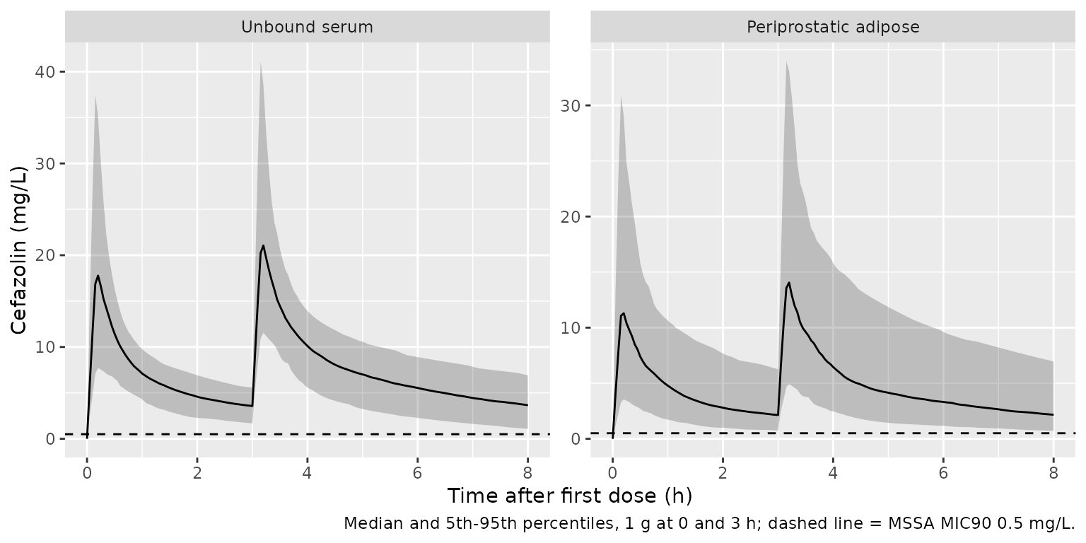
Periprostatic adipose concentration at prostate removal
The Discussion reports a mean periprostatic adipose concentration of 4.54 ug/g across all 67 samples, more than 80% of which followed a 1 g dose. Figure 1b places most tissue samples between 1 and 2 h after dosing. The simulated mean over that window, weighted 59:8 across the 1 g and 2 g arms as in the study, is compared below. Sampling times are not tabulated, so this is a coarse structural check: a mis-transcribed volume or partition coefficient moves it by tens of percent.
tissue <- sim_surg |>
  filter(time >= 1, time <= 2) |>
  group_by(arm) |>
  summarise(mean_Cadipose = mean(Cadipose), .groups = "drop")
w <- c("1 g" = 59, "2 g" = 8)
tissue_mean <- sum(tissue$mean_Cadipose * w[tissue$arm]) / sum(w)
tissue |>
  bind_rows(tibble(arm = "Study mix (59:8)", mean_Cadipose = tissue_mean)) |>
  mutate(mean_Cadipose = round(mean_Cadipose, 2)) |>
  rename(Arm = arm, `Simulated mean Cadipose 1-2 h (mg/L)` = mean_Cadipose) |>
knitr::kable(caption = "Published mean 4.54 ug/g (Discussion; density 1 kg/L).")| Arm | Simulated mean Cadipose 1-2 h (mg/L) |
|---|---|
| 1 g | 4.06 |
| 2 g | 8.55 |
| Study mix (59:8) | 4.59 |
Probability of target attainment (Figure 4)
The paper’s Monte Carlo simulation gives a single 1 g dose as a 15-minute infusion and reports, for creatinine clearance 5-120 mL/min, the percentage of patients whose unbound serum (Figure 4a) and periprostatic adipose (Figure 4b) concentration still exceeds the MSSA MIC90 of 0.5 mg/L at 3, 5, 6, 9 and 12 h. Here 200 virtual patients are simulated at each of six creatinine-clearance levels and target attainment is computed on the individual predictions. The published percentages were digitised by the maintainers from Figure 4.
crcl_levels <- c(20, 40, 60, 80, 100, 120)
pta_cohort <- tidyr::crossing(CRCL = crcl_levels, rep = seq_len(n_arm)) |>
  mutate(id = row_number(), dose_mg = 1000) |>
  select(-rep)
events_pta <- make_events(pta_cohort, dose_times = 0, t_obs = c(3, 5, 6, 9, 12), tinf = 15 / 60)
sim_pta <- rxode2::rxSolve(mod, events = events_pta, keep = "CRCL") |>
  as.data.frame()

pta_sim <- sim_pta |>
  group_by(CRCL, time) |>
  summarise(serum = 100 * mean(Cc > 0.5), adipose = 100 * mean(Cadipose > 0.5), .groups = "drop") |>
  pivot_longer(c(serum, adipose), names_to = "matrix", values_to = "pta_sim")

# Digitised from Figure 4 (panel a = serum, panel b = adipose), percent.
pta_pub <- tibble::tribble(
  ~matrix,   ~time, ~`20`, ~`40`, ~`60`, ~`80`, ~`100`, ~`120`,
  "serum",       3,   100,   100,   100,   100,    100,    100,
  "serum",       5,   100,   100,   100,    99,     96,     91,
  "serum",       6,   100,   100,    98,    95,     92,     80,
  "serum",       9,   100,    98,    90,    74,     56,     39,
  "serum",      12,   100,    89,    60,    42,     23,     13,
  "adipose",     3,   100,   100,   100,    99,     97,     96,
  "adipose",     5,   100,   100,    97,    90,     85,     73,
  "adipose",     6,   100,   100,    92,    84,     71,     56,
  "adipose",     9,   100,    90,    69,    50,     35,     20,
  "adipose",    12,    96,    70,    41,    23,     13,      6
) |>
  pivot_longer(-c(matrix, time), names_to = "CRCL", values_to = "pta_pub") |>
  mutate(CRCL = as.numeric(CRCL))

pta_cmp <- inner_join(pta_sim, pta_pub, by = c("matrix", "CRCL", "time")) |>
  mutate(diff = pta_sim - pta_pub)
stopifnot(nrow(pta_cmp) == 60)

ggplot(pta_cmp, aes(CRCL, pta_sim, colour = factor(time))) +
  geom_line() +
  geom_point(aes(y = pta_pub), shape = 1, size = 2) +
  facet_wrap(~ factor(matrix, levels = c("serum", "adipose"),
                      labels = c("a: unbound serum", "b: periprostatic adipose"))) +
  labs(x = "Creatinine clearance (mL/min)", y = "Probability of target attainment (%)",
       colour = "Time (h)",
       caption = "Lines: simulated; open circles: digitised from Figure 4 of Komatsu 2026.")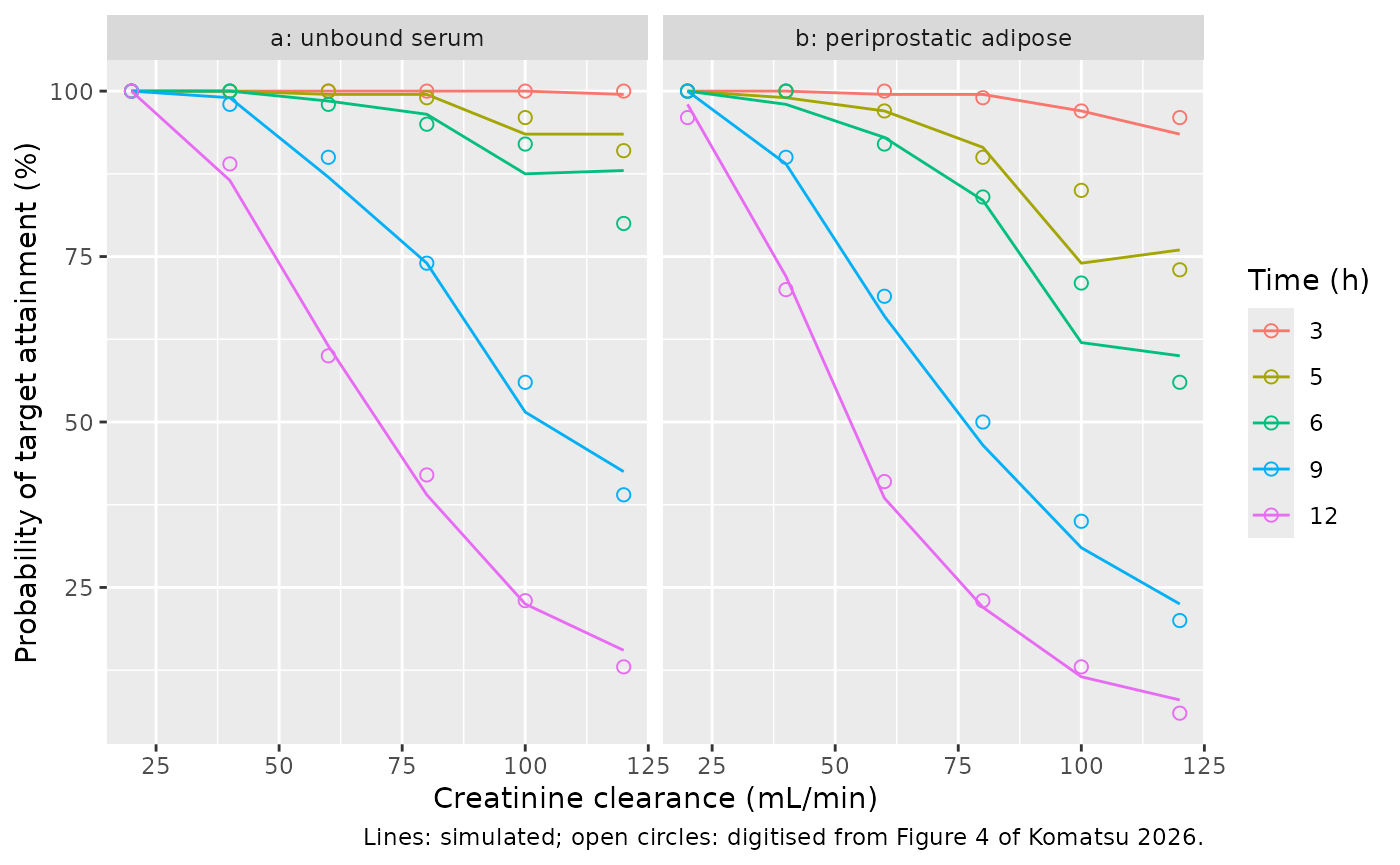
pta_cmp |>
  filter(time %in% c(5, 9, 12)) |>
  mutate(across(c(pta_sim, diff), round)) |>
  arrange(desc(matrix), time, CRCL) |>
  select(matrix, time, CRCL, pta_sim, pta_pub, diff) |>
  rename(Matrix = matrix, `Time (h)` = time, `CLcr (mL/min)` = CRCL,
         `Simulated (%)` = pta_sim, `Figure 4 (%)` = pta_pub, `Difference` = diff) |>
knitr::kable(caption = "Probability of target attainment, simulated vs Figure 4.")| Matrix | Time (h) | CLcr (mL/min) | Simulated (%) | Figure 4 (%) | Difference |
|---|---|---|---|---|---|
| serum | 5 | 20 | 100 | 100 | 0 |
| serum | 5 | 40 | 100 | 100 | 0 |
| serum | 5 | 60 | 100 | 100 | 0 |
| serum | 5 | 80 | 100 | 99 | 0 |
| serum | 5 | 100 | 94 | 96 | -2 |
| serum | 5 | 120 | 94 | 91 | 2 |
| serum | 9 | 20 | 100 | 100 | 0 |
| serum | 9 | 40 | 99 | 98 | 1 |
| serum | 9 | 60 | 87 | 90 | -3 |
| serum | 9 | 80 | 74 | 74 | 0 |
| serum | 9 | 100 | 52 | 56 | -4 |
| serum | 9 | 120 | 42 | 39 | 4 |
| serum | 12 | 20 | 100 | 100 | 0 |
| serum | 12 | 40 | 86 | 89 | -2 |
| serum | 12 | 60 | 62 | 60 | 2 |
| serum | 12 | 80 | 39 | 42 | -3 |
| serum | 12 | 100 | 22 | 23 | 0 |
| serum | 12 | 120 | 16 | 13 | 2 |
| adipose | 5 | 20 | 100 | 100 | 0 |
| adipose | 5 | 40 | 99 | 100 | -1 |
| adipose | 5 | 60 | 97 | 97 | 0 |
| adipose | 5 | 80 | 92 | 90 | 2 |
| adipose | 5 | 100 | 74 | 85 | -11 |
| adipose | 5 | 120 | 76 | 73 | 3 |
| adipose | 9 | 20 | 100 | 100 | 0 |
| adipose | 9 | 40 | 89 | 90 | -1 |
| adipose | 9 | 60 | 66 | 69 | -3 |
| adipose | 9 | 80 | 46 | 50 | -4 |
| adipose | 9 | 100 | 31 | 35 | -4 |
| adipose | 9 | 120 | 22 | 20 | 2 |
| adipose | 12 | 20 | 98 | 96 | 2 |
| adipose | 12 | 40 | 72 | 70 | 2 |
| adipose | 12 | 60 | 38 | 41 | -2 |
| adipose | 12 | 80 | 22 | 23 | -1 |
| adipose | 12 | 100 | 12 | 13 | -2 |
| adipose | 12 | 120 | 8 | 6 | 2 |
The headline conclusions reproduce: target attainment in serum exceeds 90% at 3 h for every creatinine clearance, and stays above 90% at 5 h for creatinine clearance up to 80 mL/min.
# Each simulated cell carries up to ~3.5 points of binomial error and each
# digitised cell ~2. A mis-transcribed CL, exponent, Vc or FPA shifts the
# 9 h and 12 h cells by 10-40 points.
stopifnot(
  abs(median(pta_cmp$diff)) < 4,
  quantile(abs(pta_cmp$diff), 0.9) < 10
)
serum_5h <- pta_sim |> filter(matrix == "serum", time == 5, CRCL <= 80)
serum_3h <- pta_sim |> filter(matrix == "serum", time == 3)
stopifnot(all(serum_3h$pta_sim > 90), all(serum_5h$pta_sim > 90))
PKNCA validation
The paper reports no NCA. A single-dose simulation (10-minute infusion of 1 g or 2 g, sampled to 24 h) is analysed with PKNCA and the resulting clearance is checked against each subject’s own model clearance, which validates the simulation set-up (dose, units, infusion) end to end.
t_nca <- sort(unique(c(0, 0.1, 0.17, 0.25, 0.5, 0.75, 1, 1.5, 2, 3, 4, 5, 6, 8, 10, 12, 16, 20, 24)))
events_sd <- make_events(cohort, dose_times = 0, t_obs = t_nca, tinf = 10 / 60)
sim_sd <- rxode2::rxSolve(mod, events = events_sd, keep = c("arm", "CRCL")) |>
  as.data.frame()

sim_nca <- sim_sd |>
  filter(!is.na(Cc)) |>
  select(id, time, Cc, arm)
sim_nca <- bind_rows(sim_nca, sim_nca |> distinct(id, arm) |> mutate(time = 0, Cc = 0)) |>
  distinct(id, arm, time, .keep_all = TRUE) |>
  arrange(id, time)

conc_obj <- PKNCA::PKNCAconc(sim_nca, Cc ~ time | arm + id)
dose_df <- events_sd |>
  filter(evid == 1) |>
  mutate(duration = amt / rate) |>
  select(id, time, amt, duration, arm)
dose_obj <- PKNCA::PKNCAdose(dose_df, amt ~ time | arm + id, route = "intravascular",
                             duration = "duration")
intervals <- data.frame(start = 0, end = Inf, cmax = TRUE, aucinf.obs = TRUE,
                        cl.obs = TRUE, half.life = TRUE)
nca_res <- PKNCA::pk.nca(PKNCA::PKNCAdata(conc_obj, dose_obj, intervals = intervals))

nca_df <- as.data.frame(nca_res)
nca_df |>
  filter(PPTESTCD %in% c("cmax", "aucinf.obs", "cl.obs", "half.life")) |>
  group_by(arm, PPTESTCD) |>
  summarise(median = signif(median(PPORRES, na.rm = TRUE), 3), .groups = "drop") |>
  pivot_wider(names_from = PPTESTCD, values_from = median) |>
  rename(Arm = arm, `Cmax (mg/L)` = cmax, `AUC0-inf (mg*h/L)` = aucinf.obs,
         `CL (L/h)` = cl.obs, `t1/2 (h)` = half.life) |>
knitr::kable(caption = "Median single-dose NCA of unbound serum cefazolin.")| Arm | AUC0-inf (mg*h/L) | CL (L/h) | Cmax (mg/L) | t1/2 (h) |
|---|---|---|---|---|
| 1 g | 40.2 | 24.9 | 19.9 | 3.16 |
| 2 g | 79.5 | 25.1 | 38.5 | 3.32 |
cl_check <- nca_df |>
  filter(PPTESTCD == "cl.obs") |>
  select(id, cl_nca = PPORRES) |>
  inner_join(sim_sd |> distinct(id, cl), by = "id") |>
  mutate(pct = 100 * (cl_nca / cl - 1))
# Same drawn parameters on both sides; the difference is the trapezoidal and
# extrapolation error of a 19-point grid, a few percent at most.
stopifnot(
  nrow(cl_check) == 2 * n_arm,
  abs(median(cl_check$pct)) < 3,
  quantile(abs(cl_check$pct), 0.9) < 6
)
Unbound clearance and volumes are several-fold the total-drug values usually reported for cefazolin, because about 80-90% of cefazolin is protein bound. The typical-value terminal half-life implied by Table 2 at 69 mL/min is about 3.1 h (the median NCA half-life above is similar); this is longer than the 1.8-2 h generic cefazolin half-life that the Discussion cites from the literature.
Assumptions and deviations
-
One residual error for both matrices. Table 2
reports a single proportional residual error (21.6%) for the joint serum
and tissue fit. It is carried as two parameters with the same value,
propSdfor unbound serum andpropSd_Cadiposefor adipose tissue. - Variances from Table 2. The Table 2 footnote defines omega as the square root of the inter-individual variance; the tabulated percentages are squared to give the variances (for example 28.3% gives 0.0801).
- IIV on Q was fixed to zero by the authors and is omitted.
- Tissue units. Tissue concentrations are mg/kg, read as mg/L at the 1 kg/L density the authors assumed.
- Creatinine clearance distribution. Only the median and IQR are published; the log-normal virtual distribution is a maintainers’ assumption. Weight (which set the 1 g / 2 g dose) is not a model covariate.
- Infusion durations. The study infused over 10 minutes; the Figure 4 replication uses the 15-minute infusion of the paper’s own Monte Carlo simulations.
- Target attainment is computed on individual predictions without residual error; the paper does not say whether its NONMEM simulations included the residual term (at the cohort sizes here the two differ by a few points).
- No erratum was found for this article (checked 2026-11-12).