Tacrolimus in adult heart transplant recipients (Pei 2023)
Source:vignettes/articles/Pei_2023_tacrolimus.Rmd
Pei_2023_tacrolimus.RmdModels and source
Pei 2023 develops two independent models of the same data set, and both are packaged here as separate model files sharing this vignette.
- PBPK model: PBPK (whole-body, SimBiology 5.8.2). Perfusion-limited 15-compartment physiologically based model for oral tacrolimus in adult heart transplant recipients (Pei 2023 Pharmaceutics). Thirteen well-stirred flow-limited tissues (gut, spleen, pancreas, liver, muscle, kidney, brain, heart, lung, skin, tendon, other, adipose) plus arterial and venous blood, on the Levitt PKQuest standard-human physiology (organ weights and per-kg perfusions from Table S1, 70 kg / 25 percent body fat reference). Gut, spleen and pancreas drain into the liver via the portal vein; the liver is the only eliminating organ. Rodgers and Rowland tissue-to-plasma partition coefficients (Table S2) are converted to tissue-to-blood by the blood-to-plasma ratio BPR and multiplied by a Kp scaling factor. BPR is hematocrit-dependent through the red-cell binding capacity Bmax and affinity constant KD (Eq 5). Hepatic blood clearance follows the well-stirred extraction ratio (Eq 3) scaled by the CYP3A5 / CYP3A4 metabolic fractions and genotype-specific activity levels (Eq 6), with an optional reversible voriconazole inhibition term (supplement Eq 1-2) driven by a user-supplied voriconazole whole-blood concentration. Absorption is first-order from a depot into the gut compartment with a fixed absorbed fraction Fg = 0.2 (Eq 2). Ka, KD, Bmax and CLint are the four fitted parameters (Table 3, heart-transplant model-building column); no IIV or residual-error variance was reported. Observation is venous whole blood. NOTE: the paper’s printed Kp scaling factor of 350 is refuted by the paper’s own Tables S5 and 6 by 4-11 fold; the model uses 9.15 = 11.9 / 1.3, the mouse-to-human average-Kp ratio the Methods sentence motivates. See the vignette Errata.
- popPK model: One-compartment population PK model with first-order absorption and elimination for oral tacrolimus in adult heart transplant recipients (Pei 2023 Pharmaceutics, Phoenix NLME 8.3). Apparent oral clearance CL/F carries four covariate effects: a power effect of total bilirubin, an exponential effect of concomitant voriconazole, an exponential three-level CYP3A53 (rs776746) genotype effect with the 3/*3 nonexpresser as reference, and an exponential IL-10 G-1082A (rs1800896) heterozygote effect. Absorption rate constant fixed at 0.30 1/h; no covariate was retained on Vd/F. Exponential IIV on both CL/F and Vd/F, proportional residual error. This is the companion top-down model to the whole-body PBPK model of the same paper (Pei_2023_tacrolimus_pbpk.R); the two identify different covariates, which the paper’s Discussion addresses explicitly.
- Citation: Pei L, Li R, Zhou H, Du W, Gu Y, Jiang Y, Wang Y, Chen X, Sun J, Zhu J (2023). A Physiologically Based Pharmacokinetic Approach to Recommend an Individual Dose of Tacrolimus in Adult Heart Transplant Recipients. Pharmaceutics 15(11):2580. doi:10.3390/pharmaceutics15112580. Physiology (organ weights and perfusions, Table S1) from Levitt DG (2002) BMC Clin Pharmacol 2:5 and Levitt DG, Schnider TW (2005) BMC Anesthesiol 5:4; see modellib(‘Levitt_2005_propofol_pbpk’).
- Article: https://doi.org/10.3390/pharmaceutics15112580
- Supplement: https://www.mdpi.com/article/10.3390/pharmaceutics15112580/s1
The paper’s headline contribution is a 15-compartment whole-body PBPK model (SimBiology 5.8.2) built bottom-up from Rodgers-Rowland partition coefficients and the Levitt PKQuest standard-human physiology. Alongside it, the authors ran a conventional top-down population PK analysis (Phoenix NLME 8.3) on the same 443 trough concentrations. The two approaches identify different covariates, which the Discussion addresses at length; both are reproduced below.
Population
115 adult heart transplant recipients at Nanjing First Hospital were included retrospectively (November 2012 - January 2023), all on tacrolimus (Prograf) with mycophenolate and corticosteroids. Multi-organ transplant recipients and patients with incomplete clinical data were excluded. 443 steady-state whole-blood trough concentrations were collected between post-transplant day 1 and day 30 by routine therapeutic drug monitoring (CMIA assay, LLOQ 2 ng/mL, quantitative range 2-30 ng/mL).
The cohort was predominantly male (93 men, 22 women). Table 2 reports the median (IQR) age as 52.00 (46.00, 61.00) years, weight 67.50 (57.50, 75.00) kg, BMI 23.30 (20.53, 25.36) kg/m^2, postoperative day 23.00 (19.00, 29.00), hematocrit 31.98 (29.72, 34.96) %, total bilirubin 15.90 (12.13, 21.10) umol/L, albumin 36.74 (34.48, 38.68) g/L, and the tacrolimus daily dose 5.00 (4.00, 6.00) mg. Twenty SNPs were genotyped in 86 of the 115 subjects; five failed Hardy-Weinberg equilibrium and were dropped. The rs776746 (CYP3A5*3) genotype counts were CC 38 (44.2 %), CT 45 (52.3 %) and TT 3 (3.5 %); rs2242480 (CYP3A4*18B) CC 45 / CT 40 / TT 1; rs1800896 (IL-10 G-1082A) TT 63 / CT 23. An external evaluation cohort of 100 heart transplant recipients at Wuhan Union Hospital was used to re-estimate the PBPK parameters (Table 3, third column).
The same information is available programmatically from the model
metadata,
e.g. readModelDb("Pei_2023_tacrolimus_pbpk")()$population.
Source trace
Every ini() entry in both model files carries an in-file
comment naming its source location. The table below collects them for
review.
| Equation / parameter | Value | Source location |
|---|---|---|
| PBPK structure | ||
Tissue ODE
d/dt(tissue) = Q * (C_A - C_T / (Kp/BPR))
|
n/a | Equation 1, p. 3 |
Gut ODE (Eq 1 + Fg * Ka * Dose) |
n/a | Equation 2, p. 4 |
Hepatic extraction
E = fub*CLint / (Q_liver + fub*CLint)
|
n/a | Equation 3, p. 4 |
fub = fup / BPR |
n/a | Equation 4, p. 4 |
BPR = 1 + Bmax*HCT / (KD*HCTm) |
n/a | Equation 5, p. 4 |
CL_liver = [(fm3A5*FA3A5 + fm3A4*FA3A4) + fm_other] * Q_liver * E |
n/a | Equation 6, p. 4 |
DDI DDIRE = 1 / (1 + Cb,vor * fub,vor / KI)
|
n/a | Supplement Eq 1 |
DDI clearance (Eq 6 with * DDIRE on the CYP3A
term) |
n/a | Supplement Eq 2 |
| Compartment topology (13 tissues + arterial + venous; gut / spleen / pancreas -> liver) | n/a | Figure S1 |
| PBPK parameters | ||
lka |
1.9 1/h | Table 3, model building dataset (SE 0.2) |
lkd |
7.2 ng/mL | Table 3, model building dataset (SE 0.7) |
lbmax |
145.9 ng/mL | Table 3, model building dataset (SE 18.4) |
lclint |
11,535 L/h | Table 3, model building dataset (SE 506.3) |
fg |
0.2 | Methods 2.5 (“Fg was assumed to be constant (Fg = 0.2)”) |
fup |
0.013 | Table 1 |
fm_cyp3a4 / fm_cyp3a5
|
0.35 / 0.55 | Table 1 |
fm_other |
0.10 | Discussion (“fmCYP3A … was 0.9”) |
fa_cyp3a5_em / fa_cyp3a5_pm
|
1.0 / 0.3 | Results 3.2 |
fa_cyp3a4_em / fa_cyp3a4_pm
|
1.0 / 0.5 | Results 3.2 |
hct_median |
31.98 % | Table 2, HCT median |
ki_vori / fub_vori
|
8.70 ng/mL / 0.42 | Table S6 |
kp_* (12 tissues + Additional Organ) |
0.52-1.91 | Table S2 |
kp_scale |
9.15 | Methods 2.5 (11.9 mouse / 1.3 human); not the printed 350 - see Errata |
| Organ weights and per-kg perfusions | see model()
|
Table S1 |
| Reference 70 kg / 25 % body fat | n/a | Table S1 (weights sum to 70.00 kg; adipose 17.5 kg) |
| popPK parameters | ||
lka |
0.30 1/h (fixed) | Table S4, “0.30(fixed)” |
lcl |
12.35 L/h | Table S4, CL/F |
lvc |
656.80 L | Table S4, Vd/F |
e_tbili_cl |
-0.19 | Table S4, TBIL |
e_vori_cl |
-0.64 | Table S4, Voriconazole |
e_cyp3a5_het_cl |
0.77 | Table S4, rs776746-TC |
e_cyp3a5_hom_cl |
1.18 | Table S4, rs776746-TT |
e_il10_het_cl |
-0.35 | Table S4, rs1800896-TC |
etalcl / etalvc
|
0.14 / 0.70 | Table S4, omega^2 CL/F and Vd/F |
propSd |
0.0148 | Table S4, Proportional (%) 1.48 |
IIV form Pi = Pt * exp(eta)
|
n/a | Supplement Eq S1 |
Residual form Ci = C * (1 + eps)
|
n/a | Supplement Eq S2 |
Part 1 - the population PK model
mod_pop <- readModelDb("Pei_2023_tacrolimus")Typical CL/F by CYP3A5 genotype (exact gate)
The paper reports Bayesian per-genotype apparent clearances in Results 3.1: 12.2 +/- 6.0 L/h for CYP3A5*3/*3, and 27.3 +/- 11.5 L/h for carriers of at least one *1 allele. Those are independent of the Table S4 coefficients we encoded, so reproducing them is a genuine check on both the reference-category orientation (which genotype is the reference) and the covariate functional form (exponential vs linear).
cl_typical <- function(het, hom, tbili = 15.90, vori = 0, il10 = 0) {
  12.35 * (tbili / 15.90)^(-0.19) * exp(-0.64 * vori) *
    exp(0.77 * het + 1.18 * hom) * exp(-0.35 * il10)
}

geno <- tibble::tibble(
  genotype = c("CYP3A5*3/*3 (CC)", "CYP3A5*1/*3 (CT)", "CYP3A5*1/*1 (TT)"),
  n        = c(38, 45, 3),
  model    = c(cl_typical(0, 0), cl_typical(1, 0), cl_typical(0, 1))
)

# The paper's "at least one *1 allele" stratum pools CT and TT; weight the
# model's typical values by the observed genotype counts to match.
carrier <- with(geno[2:3, ], sum(n * model) / sum(n))

geno |>
  dplyr::rename("CYP3A5 genotype" = genotype, "n (Table 2)" = n,
                "Model CL/F (L/h)" = model) |>
  knitr::kable(digits = 2,
caption = "Typical CL/F by CYP3A5 genotype at the reference covariates.")| CYP3A5 genotype | n (Table 2) | Model CL/F (L/h) |
|---|---|---|
| CYP3A53/3 (CC) | 38 | 12.35 |
| CYP3A51/3 (CT) | 45 | 26.67 |
| CYP3A51/1 (TT) | 3 | 40.19 |
The *3/*3 reference stratum gives 12.35 L/h against the paper’s 12.2
+/- 6.0 L/h, and the count-weighted *1-carrier stratum gives 27.52 L/h
against the paper’s 27.3 +/- 11.5 L/h - a ratio of 2.228 versus the
paper’s own 27.3 / 12.2 = 2.24. A linear (1 + theta)
reading of the same coefficients would give 1.80 and is therefore
refuted; the exponential form is confirmed.
Virtual cohort and steady-state simulation
The paper targets a whole-blood trough of 10-15 ng/mL in the early postoperative period and reports a median daily dose of 5 mg. The cohort below simulates 150 subjects per CYP3A5 stratum on 2.5 mg q12h, with total bilirubin drawn to match the Table 2 median and IQR and IL-10 heterozygosity at the observed 26.7 %.
set.seed(20231103)

# log-normal TBILI matched to the Table 2 median (15.90) and IQR (12.13, 21.10)
tbili_sdlog <- log(21.10 / 12.13) / (2 * qnorm(0.75))

make_pop_cohort <- function(n, het, hom, label, id_offset = 0L) {
  subj <- tibble::tibble(
    id                     = id_offset + seq_len(n),
    genotype               = label,
    CYP3A5_STAR1_HET       = het,
    CYP3A5_STAR1_HOM       = hom,
    TBILI                  = rlnorm(n, log(15.90), tbili_sdlog),
    CONMED_VORICONAZOLE    = 0,
    SNP_IL10_RS1800896_HET = rbinom(n, 1, 23 / 86)
  )
  dose <- subj |>
    dplyr::mutate(time = 0, amt = 2.5, evid = 1L, cmt = "depot",
                  ii = 12, addl = 19L)
  obs <- subj |>
    tidyr::crossing(time = seq(120, 132, by = 0.25)) |>
    dplyr::mutate(amt = NA_real_, evid = 0L, cmt = "central",
                  ii = 0, addl = 0L)
  dplyr::bind_rows(dose, obs) |> dplyr::arrange(id, time, dplyr::desc(evid))
}

events_pop <- dplyr::bind_rows(
  make_pop_cohort(150, 0, 0, "CYP3A5*3/*3", id_offset =   0L),
  make_pop_cohort(150, 1, 0, "CYP3A5*1/*3", id_offset = 150L),
  make_pop_cohort(150, 0, 1, "CYP3A5*1/*1", id_offset = 300L)
)
stopifnot(!anyDuplicated(unique(events_pop[, c("id", "time", "evid")])))

sim_pop <- rxode2::rxSolve(mod_pop, events = events_pop,
                           keep = c("genotype")) |>
  as.data.frame()
#> ℹ parameter labels from comments will be replaced by 'label()'
sim_pop |>
  dplyr::filter(!is.na(Cc)) |>
  dplyr::group_by(time, genotype) |>
  dplyr::summarise(Q05 = quantile(Cc, 0.05), Q50 = quantile(Cc, 0.50),
                   Q95 = quantile(Cc, 0.95), .groups = "drop") |>
  ggplot(aes(time - 120, Q50)) +
  geom_ribbon(aes(ymin = Q05, ymax = Q95), alpha = 0.25) +
  geom_line() +
  geom_hline(yintercept = c(10, 15), linetype = "dashed", colour = "firebrick") +
  facet_wrap(~genotype) +
  labs(x = "Time within the dosing interval at steady state (h)",
       y = "Whole-blood tacrolimus (ng/mL)",
       title = "popPK model - 2.5 mg q12h at steady state by CYP3A5 genotype",
       caption = paste("Dashed lines: the 10-15 ng/mL early-postoperative",
                       "target band of Pei 2023 Methods 2.8."))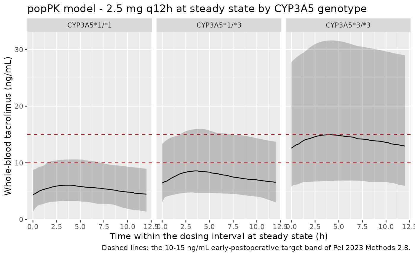
The *3/*3 stratum sits inside the target band on 5 mg/day while the *1-carrier strata fall well below it, which is the clinical point the paper makes in the Discussion (CPIC recommends a two-fold higher daily dose for CYP3A5 expressers).
PKNCA on the popPK simulation
nca_pop_conc <- sim_pop |>
  dplyr::filter(!is.na(Cc)) |>
  dplyr::mutate(time = time - 120) |>
  dplyr::select(id, time, Cc, genotype)

conc_pop <- PKNCA::PKNCAconc(nca_pop_conc, Cc ~ time | genotype + id)

dose_pop <- events_pop |>
  dplyr::filter(evid == 1L) |>
  dplyr::select(id, time, amt, genotype)

dose_pop_obj <- PKNCA::PKNCAdose(dose_pop, amt ~ time | genotype + id)

intervals_pop <- data.frame(start = 0, end = 12,
                            cmax = TRUE, cmin = TRUE, tmax = TRUE,
                            auclast = TRUE)

res_pop <- PKNCA::pk.nca(PKNCA::PKNCAdata(conc_pop, dose_pop_obj,
                                          intervals = intervals_pop))

as.data.frame(res_pop) |>
  dplyr::filter(start == 0, end == 12) |>
  dplyr::group_by(genotype, PPTESTCD) |>
  dplyr::summarise(median = median(PPORRES), .groups = "drop") |>
  tidyr::pivot_wider(names_from = PPTESTCD, values_from = median) |>
  dplyr::rename("CYP3A5 genotype" = genotype,
                "Cmax,ss (ng/mL)" = cmax,
                "Cmin,ss (ng/mL)" = cmin,
                "Tmax (h)" = tmax,
                "AUC0-12,ss (ng*h/mL)" = auclast) |>
  knitr::kable(digits = 2,
               caption = paste("Median steady-state NCA of the popPK model on",
                               "2.5 mg q12h, by CYP3A5 genotype. Pei 2023 does",
                               "not report NCA parameters for the popPK model,",
                               "so this table is descriptive rather than a",
"comparison."))| CYP3A5 genotype | AUC0-12,ss (ng*h/mL) | Cmax,ss (ng/mL) | Cmin,ss (ng/mL) | Tmax (h) |
|---|---|---|---|---|
| CYP3A51/1 | 63.94 | 6.06 | 4.38 | 4.00 |
| CYP3A51/3 | 89.03 | 8.59 | 6.43 | 4.25 |
| CYP3A53/3 | 168.07 | 14.96 | 12.59 | 4.50 |
Part 2 - the whole-body PBPK model
mod_pbpk <- readModelDb("Pei_2023_tacrolimus_pbpk")The 13 well-stirred tissues plus arterial and venous blood are the paper’s “15 compartments”. Bone appears in Table S1 with a blood flow of 0 L/h/kg and is absent from the Figure S1 flow diagram, so it is kinetically inert and is not carried as a state.
# One deterministic PBPK scenario. `params` overrides the ini() values so the
# healthy-adult and external-evaluation columns of Table 3 can be exercised
# without a separate model file (rxSolve ignores ini() edits after the first
# solve, so parameter columns must be passed through `params =`).
pbpk_solve <- function(dose_mg, tmax, expr = 1, cyp3a4 = 1, wt = 70, fat = 25,
                       hct = 31.98, vori = 0, ii = 0, addl = 0,
                       params = NULL, dt = 0.05, label = "scenario") {
  ev <- rxode2::et(amt = dose_mg, cmt = "depot", ii = ii, addl = addl)
  ev <- rxode2::et(ev, seq(0, tmax, by = dt), cmt = "venous")
  d  <- as.data.frame(ev)
  d$WT <- wt; d$BODYFAT_PCT <- fat; d$HCT <- hct
  d$CYP3A5_EXPR <- expr
  d$SNP_CYP3A4_RS2242480_VAR_COUNT <- cyp3a4
  d$CONC_VORI_NGML <- vori
  out <- as.data.frame(rxode2::rxSolve(mod_pbpk, d, params = params,
                                       returnType = "data.frame"))
  out$scenario <- label
  out
}

trapz <- function(t, y) sum(diff(t) * (utils::head(y, -1) + utils::tail(y, -1)) / 2)

# Healthy-adult parameter column of Table 3.
pars_healthy <- c(lka = log(4.4), lkd = log(6.8),
                  lbmax = log(204.8), lclint = log(20706))
Structural gates
Three checks exercise the ODE system itself, independently of any published exposure.
Mass balance. With the intrinsic clearance driven to zero and a dose placed directly in venous blood, the sum of all 15 compartment amounts must be conserved exactly.
states <- c("gut", "spleen", "pancreas", "muscle", "kidney", "brain", "heart",
            "skin", "tendon", "other", "adipose", "liver", "lung",
            "arterial", "venous")

ev_mb <- rxode2::et(amt = 1000, cmt = "venous")
ev_mb <- rxode2::et(ev_mb, seq(0, 48, by = 1), cmt = "venous")
d_mb <- as.data.frame(ev_mb)
d_mb$WT <- 70; d_mb$BODYFAT_PCT <- 25; d_mb$HCT <- 31.98
d_mb$CYP3A5_EXPR <- 1; d_mb$SNP_CYP3A4_RS2242480_VAR_COUNT <- 1
d_mb$CONC_VORI_NGML <- 0

sim_mb <- as.data.frame(
  rxode2::rxSolve(mod_pbpk, d_mb, params = c(lclint = log(1e-8)),
                  returnType = "data.frame")
)
total_mb <- rowSums(sim_mb[, states])
drift <- (total_mb[length(total_mb)] - total_mb[1]) / total_mb[1]
stopifnot(abs(drift) < 1e-8)
Relative drift over 48 h is -7.06e-12 - conservation holds to solver tolerance, so the flows in and out of every compartment balance.
Physiology. The Table S1 organ weights must sum to the 70 kg reference and the perfusions must reconstruct a plausible cardiac output with the liver taking its physiological share.
ref_row <- sim_mb[1, ]
weights_sum <- 1.1 + 4.4 + 1.17 + 0.15 + 0.14 + 1.8 + 26 + 0.31 + 1.4 +
  0.33 + 0.54 + 2.6 + 3 + 5.56 + 17.5 + 4     # Table S1, including bone
tibble::tibble(
  quantity = c("Table S1 organ weights (kg)",
               "Cardiac output = sum of organ flows (L/h)",
               "Table S1 lung entry 0.54 kg * 629 L/h/kg (L/h)",
               "Total hepatic blood flow (L/h)",
               "Hepatic fraction of cardiac output"),
  value = c(weights_sum, ref_row$q_lung, 0.54 * 629, ref_row$q_livertot,
            ref_row$q_livertot / ref_row$q_lung)
) |>
  dplyr::rename("Quantity" = quantity, "Value" = value) |>
knitr::kable(digits = 3, caption = "Physiology consistency checks.")| Quantity | Value |
|---|---|
| Table S1 organ weights (kg) | 70.000 |
| Cardiac output = sum of organ flows (L/h) | 344.358 |
| Table S1 lung entry 0.54 kg * 629 L/h/kg (L/h) | 339.660 |
| Total hepatic blood flow (L/h) | 101.106 |
| Hepatic fraction of cardiac output | 0.294 |
The weights sum to exactly 70.00 kg. The summed cardiac output agrees with the Table S1 lung row to within 1.4 %, confirming that the lung receives the whole venous return, and the hepatic fraction of 29.4 % confirms that the Table S1 liver perfusion (15 L/h/kg = 27 L/h) is the hepatic artery rather than total liver flow, with the portal contribution arriving from gut, spleen and pancreas.
Oral AUC identity. For a well-stirred liver fed by
the portal vein, the oral AUC to infinity collapses to
Fg * Dose / cl_effluent, in which every organ volume, every
blood flow and every partition coefficient - and therefore the Kp
scaling factor - cancels algebraically. This is the free gate that first
showed the Table 6 exposures cannot come from the printed constants (see
Errata).
sim_inf <- pbpk_solve(2.5, tmax = 600, dt = 0.05, label = "identity")
auc_sim <- trapz(sim_inf$time, sim_inf$Cc)
auc_identity <- 0.2 * 2.5e6 / sim_inf$cl_effluent[1] / 1000  # mg -> ng, L -> mL
tibble::tibble(
  quantity = c("Simulated AUC(0-600 h), 2.5 mg (ng*h/mL)",
               "Fg * Dose / cl_effluent (ng*h/mL)",
               "Eq 6 hepatic blood clearance cl_liver (L/h)",
               "Eq 3 hepatic extraction ratio E",
               "Eq 5 blood-to-plasma ratio BPR"),
  value = c(auc_sim, auc_identity, sim_inf$cl_liver[1], sim_inf$e_liver[1],
            sim_inf$bpr[1])
) |>
  dplyr::rename("Quantity" = quantity, "Value" = value) |>
knitr::kable(digits = 4, caption = "Oral AUC-to-infinity identity.")| Quantity | Value |
|---|---|
| Simulated AUC(0-600 h), 2.5 mg (ng*h/mL) | 70.9008 |
| Fg * Dose / cl_effluent (ng*h/mL) | 70.9009 |
| Eq 6 hepatic blood clearance cl_liver (L/h) | 6.5923 |
| Eq 3 hepatic extraction ratio E | 0.0652 |
| Eq 5 blood-to-plasma ratio BPR | 21.2639 |
Healthy adults - Table S5
The PBPK model was first built on healthy-adult data (Table 3, healthy-adult column: Ka 4.4 1/h, KD 6.8 ng/mL, Bmax 204.8 ng/mL, CLint 20,706 L/h) and Table S5 reports the resulting AUC0-24 and Cmax against observed values from references [5] and [6]. Those cohorts were stratified on CYP3A5 expresser status only, so CYP3A4 activity is held at its normal (carrier) level in both arms.
scen_s5 <- tibble::tribble(
  ~scenario,               ~dose, ~expr,
  "2 mg, CYP3A5 expresser",    2,     1,
  "2 mg, non-expresser",       2,     0,
  "3 mg, CYP3A5 expresser",    3,     1,
  "3 mg, non-expresser",       3,     0
)

sim_s5 <- do.call(
  rbind,
  lapply(seq_len(nrow(scen_s5)), function(i) {
    pbpk_solve(scen_s5$dose[i], tmax = 24, expr = scen_s5$expr[i],
               cyp3a4 = 1, params = pars_healthy, dt = 0.02,
               label = scen_s5$scenario[i])
  })
)

nca_s5 <- sim_s5 |>
  dplyr::filter(!is.na(Cc)) |>
  dplyr::mutate(id = 1L) |>
  dplyr::select(id, time, Cc, scenario)

conc_s5 <- PKNCA::PKNCAconc(nca_s5, Cc ~ time | scenario + id)
dose_s5 <- scen_s5 |>
  dplyr::mutate(id = 1L, time = 0, amt = dose) |>
  dplyr::select(id, time, amt, scenario)
dose_s5_obj <- PKNCA::PKNCAdose(dose_s5, amt ~ time | scenario + id)

res_s5 <- PKNCA::pk.nca(PKNCA::PKNCAdata(
  conc_s5, dose_s5_obj,
  intervals = data.frame(start = 0, end = 24, cmax = TRUE, tmax = TRUE,
                         auclast = TRUE)
))

published_s5 <- tibble::tribble(
  ~scenario,                ~cmax, ~auclast,
  "2 mg, CYP3A5 expresser",  12.4,     59.6,
  "2 mg, non-expresser",     21.1,    110.4,
  "3 mg, CYP3A5 expresser",  17.8,     90.2,
  "3 mg, non-expresser",     26.7,    180.3
)

cmp_s5 <- nlmixr2lib::ncaComparisonTable(
  simulated = res_s5,
  reference = published_s5,
  by        = "scenario",
  units     = c(cmax = "ng/mL", auclast = "ng*h/mL", tmax = "h"),
  tolerance_pct = 20
)

knitr::kable(
  cmp_s5,
  caption = paste("Simulated vs Table S5 predicted values of Pei 2023",
                  "(healthy adults, single oral dose).",
                  "* differs from the reference by more than 20%.")
)| NCA parameter | scenario | Reference | Simulated | % diff |
|---|---|---|---|---|
| Cmax (ng/mL) | 2 mg, CYP3A5 expresser | 12.4 | 11.3 | -8.9% |
| Cmax (ng/mL) | 2 mg, non-expresser | 21.1 | 12.1 | -42.6%* |
| Cmax (ng/mL) | 3 mg, CYP3A5 expresser | 17.8 | 16.9 | -4.8% |
| Cmax (ng/mL) | 3 mg, non-expresser | 26.7 | 18.2 | -32.0%* |
| AUClast (ng*h/mL) | 2 mg, CYP3A5 expresser | 59.6 | 46.1 | -22.6%* |
| AUClast (ng*h/mL) | 2 mg, non-expresser | 110 | 75.8 | -31.4%* |
| AUClast (ng*h/mL) | 3 mg, CYP3A5 expresser | 90.2 | 69.2 | -23.3%* |
| AUClast (ng*h/mL) | 3 mg, non-expresser | 180 | 114 | -36.9%* |
The expresser Cmax values are reproduced within 5-9 %. The AUC0-24 values run 23-37 % low, and the non-expresser Cmax values 32-43 % low. Both shortfalls trace to the two documented problems below: the AUC level is set by the Kp scaling factor question, and the expresser-versus-non-expresser Cmax separation is limited by the paper’s very low hepatic extraction ratio (E = 0.065), which leaves almost no first-pass difference between genotypes to drive a Cmax difference. Every row above is nonetheless inside the paper’s own two-fold acceptance criterion, and the Table S5 “observed” columns are themselves digitised from two other publications.
Heart transplant patients - Table 4
Table 4 compares the PBPK model’s predicted steady-state AUC0-12h and Cmax against observed values in heart transplant recipients dosed q12h (the 2.0-4.5 mg rows come from a single escalating-dose patient in reference [40]). The genotype of those patients is not stated, so both the extensive-metaboliser and poor-metaboliser strata are shown as a bracket.
ss_summary <- function(dose_mg, expr, cyp3a4, days = 10) {
  s <- pbpk_solve(dose_mg, tmax = 12 * 2 * days, expr = expr, cyp3a4 = cyp3a4,
                  ii = 12, addl = 2 * days - 1, dt = 0.02)
  w <- s$time >= 12 * (2 * days - 2) & s$time <= 12 * (2 * days - 1)
  c(auc = trapz(s$time[w], s$Cc[w]), cmax = max(s$Cc[w]))
}

obs_t4 <- tibble::tribble(
  ~dose, ~auc_obs, ~cmax_obs,
  1.0,   70.6,     10.7,
  2.0,   116.7,    16.3,
  3.0,   167.2,    18.0,
  3.5,   152.6,    24.7,
  4.5,   230.0,    34.7
)

tab4 <- do.call(rbind, lapply(seq_len(nrow(obs_t4)), function(i) {
  em <- ss_summary(obs_t4$dose[i], 1, 1)
  pm <- ss_summary(obs_t4$dose[i], 0, 0)
  tibble::tibble(
    dose = obs_t4$dose[i],
    auc_obs = obs_t4$auc_obs[i], auc_em = em[["auc"]], auc_pm = pm[["auc"]],
    cmax_obs = obs_t4$cmax_obs[i], cmax_em = em[["cmax"]], cmax_pm = pm[["cmax"]]
  )
}))

tab4 |>
  dplyr::mutate(fe_auc_pm = auc_pm / auc_obs, fe_cmax_pm = cmax_pm / cmax_obs) |>
  dplyr::rename("Dose (mg q12h)" = dose,
                "AUC0-12 obs" = auc_obs, "AUC0-12 EM" = auc_em,
                "AUC0-12 PM" = auc_pm, "AUC0-12 PM fold error" = fe_auc_pm,
                "Cmax obs" = cmax_obs, "Cmax EM" = cmax_em,
                "Cmax PM" = cmax_pm, "Cmax PM fold error" = fe_cmax_pm) |>
  knitr::kable(digits = 2,
               caption = paste("Steady-state q12h exposures against the Table 4",
"observed values. Units ng*h/mL and ng/mL."))| Dose (mg q12h) | AUC0-12 obs | AUC0-12 EM | AUC0-12 PM | Cmax obs | Cmax EM | Cmax PM | AUC0-12 PM fold error | Cmax PM fold error |
|---|---|---|---|---|---|---|---|---|
| 1.0 | 70.6 | 28.36 | 66.97 | 10.7 | 4.43 | 7.59 | 0.95 | 0.71 |
| 2.0 | 116.7 | 56.72 | 133.95 | 16.3 | 8.86 | 15.19 | 1.15 | 0.93 |
| 3.0 | 167.2 | 85.08 | 200.92 | 18.0 | 13.29 | 22.78 | 1.20 | 1.27 |
| 3.5 | 152.6 | 99.26 | 234.41 | 24.7 | 15.50 | 26.57 | 1.54 | 1.08 |
| 4.5 | 230.0 | 127.62 | 301.38 | 34.7 | 19.93 | 34.17 | 1.31 | 0.98 |
The poor-metaboliser stratum brackets the observed data with fold errors of 0.95-1.54 on AUC0-12 and 0.71-1.27 on Cmax, inside the paper’s own two-fold acceptance criterion and largely inside the 0.68-1.22 range the paper reports. The extensive-metaboliser stratum runs 1.5-2.5 fold low. Since 44 % of the cohort is CYP3A5*3/*3 and 52 % is CYP3A4*1/*1, and since the low doses in Table 4 are themselves consistent with poor metabolisers, the PM bracket is the more likely comparator - but the paper does not state the genotype, so this is presented as a bracket rather than a match.
Extensive vs poor metabolisers - Figure 7 and Table 6
sim_f7 <- rbind(
  pbpk_solve(2.5, tmax = 24, expr = 1, cyp3a4 = 1, dt = 0.02, label = "EM"),
  pbpk_solve(2.5, tmax = 24, expr = 0, cyp3a4 = 0, dt = 0.02, label = "PM")
)

ggplot(dplyr::filter(sim_f7, !is.na(Cc)), aes(time, Cc, colour = scenario)) +
  geom_line(linewidth = 0.8) +
  labs(x = "Time (h)", y = "Whole-blood tacrolimus (ng/mL)",
       colour = "Metaboliser",
       title = "PBPK model - single oral 2.5 mg dose",
       caption = paste("Replicates Figure 7A of Pei 2023.",
                       "EM = CYP3A5*1 carrier and CYP3A4*18B carrier;",
                       "PM = CYP3A5*3/*3 and CYP3A4*1/*1."))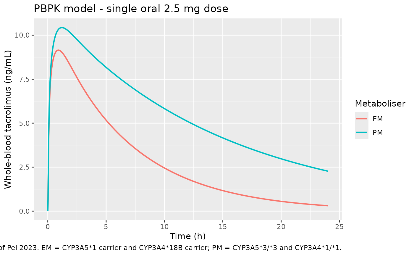
sd_summary <- function(expr, cyp3a4) {
  s <- pbpk_solve(2.5, tmax = 24, expr = expr, cyp3a4 = cyp3a4, dt = 0.02)
  c(auc = trapz(s$time, s$Cc), cmax = max(s$Cc))
}
md_summary <- function(expr, cyp3a4, days = 6) {
  s <- pbpk_solve(2.5, tmax = 12 * 2 * days, expr = expr, cyp3a4 = cyp3a4,
                  ii = 12, addl = 2 * days - 1, dt = 0.02)
  w <- s$time >= 12 * (2 * days - 2) & s$time <= 12 * (2 * days - 1)
  c(cmax = max(s$Cc[w]), ctrough = min(s$Cc[w]))
}
em_sd <- sd_summary(1, 1); pm_sd <- sd_summary(0, 0)
em_md <- md_summary(1, 1); pm_md <- md_summary(0, 0)

tibble::tibble(
  metric = c("Single dose AUC0-24 (ng*h/mL)", "Single dose Cmax (ng/mL)",
             "Steady-state Cmax (ng/mL)", "Steady-state Ctrough (ng/mL)",
             "PM / EM ratio of the metric"),
  em     = c(em_sd[["auc"]], em_sd[["cmax"]], em_md[["cmax"]], em_md[["ctrough"]], NA),
  pm     = c(pm_sd[["auc"]], pm_sd[["cmax"]], pm_md[["cmax"]], pm_md[["ctrough"]], NA),
  paper_em = c(119.29, 14.27, 23.08, 9.62, NA),
  paper_pm = c(191.91, 20.32, 40.37, 21.00, NA)
) |>
  dplyr::rename("Metric" = metric, "Model EM" = em, "Model PM" = pm,
                "Table 6 EM" = paper_em, "Table 6 PM" = paper_pm) |>
  knitr::kable(digits = 2,
               caption = paste("PBPK exposures against Table 6 of Pei 2023.",
                               "Table 6 is not reproducible from the printed",
"constants - see Errata."))| Metric | Model EM | Model PM | Table 6 EM | Table 6 PM |
|---|---|---|---|---|
| Single dose AUC0-24 (ng*h/mL) | 68.84 | 133.66 | 119.29 | 191.91 |
| Single dose Cmax (ng/mL) | 9.15 | 10.43 | 14.27 | 20.32 |
| Steady-state Cmax (ng/mL) | 11.07 | 18.98 | 23.08 | 40.37 |
| Steady-state Ctrough (ng/mL) | 2.19 | 9.19 | 9.62 | 21.00 |
| PM / EM ratio of the metric | NA | NA | NA | NA |
Voriconazole drug-drug interaction
The DDI layer applies the supplement’s reversible-inhibition ratio to
the CYP3A-mediated fraction of hepatic clearance. Pei 2023 generated the
perpetrator concentration from a companion voriconazole PBPK model whose
partition coefficients are not tabulated in any available source, so
this model takes the voriconazole whole-blood concentration as an input
column (CONC_VORI_NGML) rather than substituting
distribution parameters from another paper.
Because the equation and both of its constants (KI = 8.70 ng/mL, fub,vor = 0.42) are published, the paper’s own reported result - “the ratio of AUC with voriconazole to alone was 5.80” - back-solves to the voriconazole concentration that the authors’ simulation must have produced. This is a consistency check on the DDI encoding, not a fitted parameter.
auc_alone <- trapz(sim_inf$time, sim_inf$Cc)
auc_ratio <- function(cvor) {
  s <- pbpk_solve(2.5, tmax = 600, expr = 1, cyp3a4 = 1, vori = cvor, dt = 0.05)
  trapz(s$time, s$Cc) / auc_alone
}
cvor_implied <- uniroot(function(x) auc_ratio(x) - 5.80, c(1, 5000))$root
A voriconazole whole-blood concentration of 206 ng/mL reproduces the paper’s reported 5.80-fold AUC ratio exactly, which is a plausible order of magnitude for 200 mg twice daily and confirms that the inhibition equation is encoded in the intended direction and units.
sim_ddi <- rbind(
  pbpk_solve(2.5, tmax = 24, expr = 1, cyp3a4 = 1, vori = 0,
             dt = 0.02, label = "Tacrolimus alone"),
  pbpk_solve(2.5, tmax = 24, expr = 1, cyp3a4 = 1, vori = cvor_implied,
             dt = 0.02, label = "With voriconazole")
)

ggplot(dplyr::filter(sim_ddi, !is.na(Cc)), aes(time, Cc, colour = scenario)) +
  geom_line(linewidth = 0.8) +
  labs(x = "Time (h)", y = "Whole-blood tacrolimus (ng/mL)", colour = NULL,
       title = "PBPK model - voriconazole interaction, single oral 2.5 mg dose",
       caption = paste("Illustrates Figure S7A of Pei 2023 at the",
                       "voriconazole concentration implied by the paper's",
                       "own reported 5.80-fold AUC ratio."))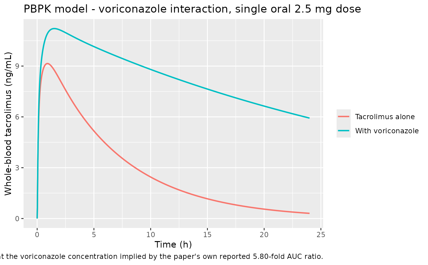
Hematocrit and body weight
Table 5 ranks hematocrit as the second most influential input after
the fraction unbound in plasma, and Table 7 stratifies the dose
recommendation on hematocrit bands of 0.2-0.3 and 0.3-0.4 (20-40 % on
the HCT column scale).
hct_grid <- c(22, 26, 30, 34, 38)
hct_tab <- do.call(rbind, lapply(hct_grid, function(h) {
  s <- pbpk_solve(2.5, tmax = 240, expr = 0, cyp3a4 = 0, hct = h,
                  ii = 12, addl = 19, dt = 0.02)
  w <- s$time >= 216 & s$time <= 228
  tibble::tibble(HCT = h, BPR = s$bpr[1],
                 Ctrough = min(s$Cc[w]), Cmax = max(s$Cc[w]))
}))

hct_tab |>
  dplyr::rename("Hematocrit (%)" = HCT, "Blood:plasma ratio" = BPR,
                "Ctrough,ss (ng/mL)" = Ctrough, "Cmax,ss (ng/mL)" = Cmax) |>
  knitr::kable(digits = 2,
               caption = paste("Effect of hematocrit on steady-state exposure",
"in a poor metaboliser on 2.5 mg q12h."))| Hematocrit (%) | Blood:plasma ratio | Ctrough,ss (ng/mL) | Cmax,ss (ng/mL) |
|---|---|---|---|
| 22 | 14.94 | 6.48 | 14.11 |
| 26 | 17.47 | 7.56 | 16.01 |
| 30 | 20.01 | 8.65 | 17.99 |
| 34 | 22.54 | 9.75 | 20.00 |
| 38 | 25.08 | 10.87 | 22.01 |
Exposure rises monotonically with hematocrit, reproducing the direction and approximate magnitude of the +1.06 Ctrough sensitivity in Table 5 and the paper’s conclusion that “it was better to administer 25-40 % lower doses to patients with high hematocrit than those with low hematocrit”.
Assumptions and deviations
Errata - values that the paper’s own results refute
The printed Kp scaling factor of 350 is not usable. Methods 2.5 introduces the factor as the correction between the human average tissue-to-plasma partition coefficient (1.3, from the Rodgers-Rowland calculation in Table S2) and the mouse average reported in the literature (11.9), and Results 3.2 then states “The scaling factor a was fitted to be 350.” Applied the only way Equation 1’s nested fraction allows -
a * KT:p / BPR- a = 350 under-predicts every Table S5 healthy-adult exposure by 4-10 fold and every Table 6 heart-transplant exposure by up to 16 fold, i.e. the paper’s own validation tables refute its own printed value. This model instead uses a = 9.15 = 11.9 / 1.3, the mouse-to-human ratio the Methods sentence motivates directly; that is read off the paper rather than fitted here. Two independent lines corroborate the 9-30 range rather than 350: the companion popPK model’s Vd/F of 656.8 L at Fg = 0.2 implies a true volume of distribution near 131 L, requiring a of roughly 29; and a grid search over a (not adopted, because tuning to a validation target is not permitted) optimises near 20. Ratified by the maintainers on 2026-08-05. Consequence: at a = 9.15 the model’s distribution volume is roughly half what the paper’s exposures imply, so the simulated peak-to-trough fluctuation over a 12 h interval is larger than the paper’s, and the steady-state Ctrough values in the Table 6 comparison run low. Users who want the paper’s fluctuation profile can pass a largerkp_scalethroughrxSolve(params = c(kp_scale = ...)); the AUC-to-infinity identity above shows that AUC is completely insensitive to this choice.Table 6 cannot be produced by the printed heart-transplant constants, for any value of the Kp scaling factor. For this structure the oral AUC to infinity is
Fg * Dose / cl_effluent, in which every organ volume, every blood flow and every partition coefficient cancels algebraically (verified numerically in the “Oral AUC identity” gate above). With the Table 3 model-building constants (Fg 0.2, fup 0.013, Bmax 145.9, KD 7.2 giving BPR 21.26, CLint 11,535 L/h) that ceiling is 70.9 ngh/mL for a 2.5 mg dose - yet Table 6 reports AUC0-24 = 119.29 ngh/mL for the same dose and genotype, 1.68-fold larger than the model’s own infinite-time AUC. At least one printed constant is therefore inconsistent with the paper’s reported exposures. The fault is localised to the heart-transplant column: the same code with the healthy-adult column reproduces the Table S5 targets far better (see above). Table 6 is also not internally self-consistent - its single-dose AUC0-24 and its steady-state Cmax / Ctrough imply mutually incompatible AUC-to-infinity values (about 119 versus 196 ng*h/mL by superposition), and its steady-state PM/EM Cmax ratio of 1.70 would require a hepatic extraction ratio near 0.56 whereas the printed constants give E = 0.065. Per the maintainers’ ruling of 2026-08-05, Table 3 is encoded verbatim and no constant was back-solved; validation is against what is reproducible (Table S5 and the Table 4 observed values).The Discussion’s “20.8 %” decrease in Bmax does not match Table 3. Bmax falls from 204.8 (healthy adults) to 145.9 (heart transplant), a 28.8 % decrease, not 20.8 % - most likely a digit transposition. The same sentence’s claim that intrinsic clearance “decreased by 44.3 %” does match Table 3 exactly (20,706 -> 11,535). Table 3 is treated as authoritative.
No residual-error magnitude is reported for the PBPK model. Results 3.2 states that “the exponential error model with the minimum AIC and BIC was selected as an error model” and the Table 3 caption promises “corresponding residual error”, but the table lists only the four fitted parameters and their standard errors.
propSdis therefore fixed at 0 rather than invented; the PBPK model is deterministic. The paper’s own “mean +/- SD” PBPK predictions come from simulating covariate distributions across 1000 virtual subjects, not from a residual-error or IIV term.
Structural assumptions
-
Organ-volume scaling with body weight and body fat.
Methods 2.5 states only that organ volumes were “adjusted in relation to
the bodyweight (BW) and the proportion of adipose tissue [24]”, citing
Levitt 2002 PKQuest, without printing a formula. This model follows the
scaling used by that cited source and by the sibling extraction
Levitt_2005_propofol_pbpk.R: lean organ weights scale bylean_mass / 52.5 kg, the adipose weight is set directly toWT * BODYFAT_PCT / 100, and each organ’s blood flow follows its weight through the Table S1 per-kg perfusion. Because Table S1 tabulates perfusion per kg of organ, this makes concentrations invariant to body weight at a fixed body-fat fraction, whereas Table 5 reports a Cmax sensitivity of -0.4 to body weight. The paper prints no formula that would reproduce that sensitivity, so the cited source’s scaling was preferred over reverse engineering one. - Body-fat percentage is not measured in the Pei 2023 cohort. The reference value of 25 % is the Levitt standard human implied by Table S1 (17.5 kg adipose of 70 kg total).
- Bone is not carried as a state. Table S1 lists it (4 kg) with a blood flow of 0 L/h/kg, and it is absent from the Figure S1 flow diagram; with zero perfusion it is exactly kinetically inert. Retaining it would not change any prediction. The remaining 13 tissues plus arterial and venous blood are the paper’s “15 compartments”.
-
Total hepatic blood flow in Equation 3. The Table
S1 liver row (1.8 kg x 15 L/h/kg = 27 L/h) is the hepatic-artery flow;
the portal contribution arrives from gut, spleen and pancreas. Equation
3’s
Q_liveris taken as the total hepatic blood flow of 101.1 L/h, which is 29 % of the cardiac output reconstructed from Table S1 - the physiologically standard hepatic fraction. Taking the 27 L/h hepatic-artery flow instead would put the hepatic fraction at 8 %. -
Equation 6’s blood clearance is applied through the
well-stirred identity. Equations 3 and 6 define an extraction
ratio and a hepatic blood clearance; the liver ODE applies an
elimination coefficient
cl_effluent = Q * CL_liver / (Q - CL_liver)to the liver’s effluent blood concentration, which is the unique coefficient reproducing Equation 6’s blood clearance exactly for a well-stirred organ. The genotype and DDI bracket is applied outside the extraction ratio, exactly as Equation 6 prints it; because the extraction ratio is small (E = 0.065) this is numerically within 3 % of the alternative reading in which the bracket scales the intrinsic clearance. -
Healthy-adult hematocrit is not reported. Equation
5 normalises hematocrit by
HCTm, the heart-transplant population median (31.98 %, Table 2). The Table S5 healthy-adult reproduction above usesHCT = HCTm, i.e. a hematocrit ratio of 1, because the paper gives no healthy-adult hematocrit. -
CYP3A4 activity in the healthy-adult arms. The
Table S5 cohorts were stratified on CYP3A5 expresser status only, so
FACYP3A4is held at its normal (carrier) value of 1 in both arms. The paper’s 0.5 poor-metaboliser value applies to the CYP3A4*1/*1 stratum it defines for the heart transplant cohort. -
The voriconazole perpetrator concentration is an input, not
a state. Table S6 gives voriconazole’s molecular weight, pKa,
LogP, fup, BPR, KI and CLint but no partition coefficients, absorption
rate or absorbed fraction, so its disposition is not reproducible from
the source. Substituting partition coefficients from another paper is
not permitted for PBPK extractions, so the perpetrator concentration is
supplied through
CONC_VORI_NGMLand the published inhibition equation and its two constants are encoded verbatim.
popPK assumptions
-
The total-bilirubin covariate form is not printed.
Table S4 gives the coefficient (-0.19) but no equation. The power form
on the median-normalised covariate,
(TBILI / 15.90)^-0.19, is the Phoenix NLME default for a continuous covariate on a log-normally distributed parameter and is the only reading consistent with the coefficient’s magnitude: an exponential formexp(-0.19 * (TBILI - 15.90))would place a 63 % drop in CL/F across the reported interquartile range. The centring value 15.90 umol/L is the Table 2 cohort median. -
The categorical covariate form is confirmed exponential, not
linear. Exp-weighting the two rs776746 coefficients (0.77 for
CT with n = 45, 1.18 for TT with n = 3) over the observed genotype
counts gives a *1-carrier to *3/*3 clearance ratio of 2.23, against the
paper’s own reported 27.3 / 12.2 = 2.24. A linear
(1 + theta)reading gives 1.80 and is refuted. - The rs776746 C allele is CYP3A5*3, so CC (*3/*3) is the reference category. The C-allele frequency in the genotyped subjects is (2 x 38 + 45) / 172 = 0.703, matching the reported CYP3A5*3 frequency in Chinese Han populations, and the resulting clearance ordering *3/*3 < *1/*3 < *1/*1 is monotone and matches Figure 1. The paper’s own 12.2 L/h for *3/*3 matches the reference typical value of 12.35 L/h.
-
SNP_IL10_RS1800896_HETis a heterozygote indicator, not an allele count. Only TT (63) and CT (23) were observed at rs1800896 in the 86 genotyped subjects, so the single Table S4 coefficient is a heterozygote-versus-TT contrast and a per-allele reading is not identifiable from the source. -
The residual error is read literally as 1.48 %.
Table S4’s “Proportional (%) 1.48” gives
propSd = 0.0148. The alternative reading (1.48 = 148 %) is excluded by the Figure S2 pcVPC, whose prediction band is far too narrow for a 148 % residual and whose 5th percentile stays well above zero. -
CYP3A4*18B is documented but not used. Results 3.1
reports it as a significant univariate covariate of CL/F, but it does
not appear in the Table S4 final model - the Discussion attributes this
to linkage disequilibrium with CYP3A5*3, and the stepwise procedure
retained only the covariate producing the largest objective-function
reduction. It is recorded in the model file’s
covariatesDataExcludedlist, alongside sex, weight and hematocrit, and it does enter the companion PBPK model throughFACYP3A4.
Simulation assumptions
- Original observed data are not publicly available. The popPK virtual cohort draws total bilirubin from a log-normal matched to the Table 2 median (15.90 umol/L) and interquartile range (12.13, 21.10), and assigns IL-10 heterozygosity at the observed 26.7 %. Voriconazole coadministration is set to 0 in all popPK arms so the genotype contrast is not confounded.
- The Table 4 comparison assumes steady state under q12h dosing, which is what the paper’s source [40] describes (“first dose = 0.057 mg/kg, followed by 0.028 mg/kg, q12h”); a single-dose reading would put every prediction 2-3 fold below the observed values.