Fesoterodine (Oishi 2014)
Source:vignettes/articles/Oishi_2014_fesoterodine.Rmd
Oishi_2014_fesoterodine.RmdModel and source
- Citation: Oishi M, Tomono Y, Yamagami H, Malhotra B. Population Pharmacokinetics of the 5-Hydroxymethyl Metabolite of Tolterodine After Administration of Fesoterodine Sustained Release Tablet in Western and East Asian Populations. Journal of Clinical Pharmacology. 2014;54(8):928-936. doi:10.1002/jcph.274
- Article: https://doi.org/10.1002/jcph.274
Oishi et al. (2014) pooled 10 pharmacokinetic and 3 efficacy/safety studies of fesoterodine sustained-release (SR) tablets across Western and East Asian populations to characterise the population pharmacokinetics of the active metabolite 5-hydroxymethyl tolterodine (5-HMT). Fesoterodine is a prodrug that is rapidly and completely converted to 5-HMT by ubiquitous nonspecific esterases; systemic 5-HMT concentrations therefore drive the muscarinic antagonism intended for the treatment of overactive bladder (OAB).
Population
The analysis dataset combined 10,922 plasma 5-HMT concentrations from 1546 subjects (Oishi 2014 Table 1, Table 2). The pooled cohort included:
- Sex: 1085 female (70.2%), 461 male (29.8%).
- CYP2D6 phenotype: 1475 extensive metabolisers (95.4%), 71 poor metabolisers (4.6%).
- Ethnicity: 878 Westerners (56.8%), 522 Japanese (33.8%), 105 Korean (6.8%), 41 other East Asian (2.7%). The final model retained only the Japanese indicator; Korean was dropped in backward elimination.
- Hepatic impairment: 8 subjects (0.5%) with Child-Pugh Class B moderate hepatic impairment, contributed exclusively by study #4. Severe hepatic impairment (Child-Pugh C) was excluded from all contributing studies.
- Concomitant CYP3A modulators: 118 subjects (7.4%) coadministered with ketoconazole (studies #1 and #6), 12 subjects (0.8%) coadministered with rifampicin (study #5).
- Age: 19-91 years (mean 55.5, SD 14.6).
- Weight: 31.2-192.8 kg (mean 70.2, SD 18.8).
- Cockcroft-Gault CRCL: 19.8-273.1 mL/min (mean 87.0, SD 30.3). A dedicated renal-impairment study (#3) contributed 24 patients across the renal-function spectrum.
- Dose range: 4-28 mg fesoterodine fumarate once daily, oral SR tablet; single- and multiple-dose regimens. Labelled doses are 4 mg and 8 mg QD.
The same information is available programmatically:
str(readModelDb("Oishi_2014_fesoterodine")()$population, max.level = 1)
#> List of 18
#>  $ species            : chr "human"
#>  $ n_subjects         : int 1546
#>  $ n_studies          : int 13
#>  $ n_observations     : int 10922
#>  $ age_range          : chr "19-91 years"
#>  $ age_median         : chr "56 years"
#>  $ weight_range       : chr "31.2-192.8 kg"
#>  $ weight_median      : chr "67.0 kg"
#>  $ sex_female_pct     : num 70.2
#>  $ race_ethnicity     : Named num [1:4] 56.8 33.8 6.8 2.7
#>   ..- attr(*, "names")= chr [1:4] "Westerner" "Japanese" "Korean" "Other Asian"
#>  $ disease_state      : chr "Pooled cohort of adult healthy volunteers and patients with overactive bladder (OAB). Contributing studies incl"| __truncated__
#>  $ dose_range         : chr "4-28 mg fesoterodine (as fesoterodine fumarate; molecular weight 527.65 g/mol) once daily as sustained-release "| __truncated__
#>  $ regions            : chr "Multi-regional pool: North America and Europe (7 Western PK studies + 2 Western OAB efficacy/safety studies); J"| __truncated__
#>  $ renal_function     : chr "Cockcroft-Gault CRCL 19.8-273.1 mL/min (mean 87.0, SD 30.3); one dedicated renal-impairment study (#3) with 24 "| __truncated__
#>  $ hepatic_function   : chr "Only Child-Pugh Class B moderate hepatic impairment enrolled (n = 8, all from study #4); severe hepatic impairm"| __truncated__
#>  $ cyp2d6_distribution: chr "Extensive metaboliser 1475 (95.4%); Poor metaboliser 71 (4.6%) (Table 2 (a))."
#>  $ conmed_distribution: chr "CYP3A inhibitor coadministration 118 (7.4%); CYP3A inducer coadministration 12 (0.8%) (Table 2 (a))."
#>  $ notes              : chr "NONMEM version V, level 1.1 with FOCEI. Structural model ADVAN2 / TRANS2 (1-cpt, first-order absorption). Preli"| __truncated__
Source trace
Every parameter’s origin is recorded as an in-file comment on its
ini() line in
inst/modeldb/specificDrugs/Oishi_2014_fesoterodine.R. The
table below collects them in one place for review; all values are drawn
from Oishi 2014 Table 3 (Final Model Parameter Estimates).
| Equation / parameter | Value | Source location |
|---|---|---|
lcl (CL/F) |
93.8 L/h | Table 3, row ‘CL/F (L/h)’. |
lvc (V/F) |
144 L | Table 3, row ‘V/F (L)’. |
lka (ka) |
0.0935 1/h | Table 3, row ‘ka (h^-1)’. |
ltlag (Tlag) |
0.447 h | Table 3, row ‘Tlag (h)’. |
e_crcl_cl (theta_5) |
0.303 | Table 3, row ‘Creatinine clearance (theta_5) on CL/F’. Applied as (CRCL/80)^0.303. |
e_hepimp_mod_cl (theta_6) |
log(0.422) | Table 3, row ‘Hepatic impairment (theta_6) on CL/F’. |
e_cyp2d6_pm_cl (theta_7) |
log(0.626) | Table 3, row ‘CYP2D6 genotype (theta_7) on CL/F’. |
e_cyp3a4_inh_cl (theta_8) |
log(0.504) | Table 3, row ‘CYP3A inhibitor (theta_8) on CL/F’. |
e_cyp3a4_ind_cl (theta_9) |
log(3.90) | Table 3, row ‘CYP3A inducer (theta_9) on CL/F’. |
e_sexf_cl (theta_11) |
log(0.903) | Table 3, row ‘Sex (theta_11) on CL/F’. |
e_race_japanese_cl (theta_13) |
log(1.12) | Table 3, row ‘Japanese (theta_13) on CL/F’. |
| IIV Var(etalcl) | 0.217 | Table 3, row ‘v^2 CL/F’ (46.6% CV). |
| IIV Var(etalvc) | 0.606 | Table 3, row ‘v^2 V/F’ (77.8% CV). |
| IIV Var(etalka) | 0.0663 | Table 3, row ‘v^2 ka’ (25.7% CV). |
| IIV Cov(etalcl, etalvc) | 0.148 | Table 3, row ‘COV CL/F-V/F’ (r = 0.408). |
| IIV Cov(etalcl, etalka) | 0.0457 | Table 3, row ‘COV CL/F-ka’ (r = 0.381). |
| IIV Cov(etalvc, etalka) | 0.0953 | Table 3, row ‘COV V/F-ka’ (r = 0.475). |
propSd |
sqrt(0.0951) = 0.30838 | Table 3, row ‘sigma^2 proportional’ (30.8% CV). |
addSd |
sqrt(0.00123) = 0.03507 | Table 3, row ‘sigma^2 additive’ (SD = 0.0351 ng/mL). |
d/dt(depot), d/dt(central),
alag(depot) <- tlag
|
1-cpt + first-order absorption + lag | Methods ‘Data Analysis’ (ADVAN2 / TRANS2 in NONMEM V, level 1.1). |
| Covariate multiplicative form | (theta_k * I + 1 * (1 - I)) |
Final model equation on p. 931-932 (Results ‘Population Pharmacokinetic Modeling Results’). |
The final model equation for CL/F (transcribed from the Results section of the paper) is
CL/F_i = theta_1 * (CRCL_i / 80)^theta_5
         * (theta_6 * HEPIMP + 1 * (1 - HEPIMP))
         * (theta_7 * CYP2D6_PM + 1 * (1 - CYP2D6_PM))
         * (theta_8 * CYP3A_inh + 1 * (1 - CYP3A_inh))
         * (theta_9 * CYP3A_ind + 1 * (1 - CYP3A_ind))
         * (theta_11 * SEXF + 1 * (1 - SEXF))
         * (theta_13 * JAPANESE + 1 * (1 - JAPANESE))
         * exp(eta_CL_i)
which is mathematically equivalent to a log-additive shift encoding
log(CL/F) = lcl + e_crcl_cl * log(CRCL / 80) + sum_k e_k_cl * I_k + etalcl
with e_k_cl = log(theta_k) for each binary covariate. The
model file uses the log-additive encoding so ini() labels
reproduce the paper’s multiplicative factors directly in the trailing
comment (e.g. log(0.422) for the hepatic impairment
shift).
Virtual cohort
Original observed data are not publicly available. The simulations below use virtual populations whose covariate distributions approximate the published trial demographics.
set.seed(2014)

# Per-arm cap: 100 subjects each. Six covariate arms are simulated to
# illustrate the covariate effects retained in the final model. The
# sampling grid is dense during the last (steady-state) dosing interval
# where NCA is computed, and sparse in the earlier accumulation phase.
n_per_arm <- 100L

make_arm <- function(name, n, id_offset,
                     CRCL = 80,
                     HEPIMP_MOD = 0L,
                     CYP2D6_PM = 0L,
                     CONMED_CYP3A4_INH = 0L,
                     CONMED_CYP3A4_IND = 0L,
                     SEXF = 0L,
                     RACE_JAPANESE = 0L,
                     dose = 8,
                     tau = 24,
                     n_doses = 7L,
                     sample_times = c(seq(0,   120, by = 6),
                                      seq(144, 168, by = 1))) {
  ids <- id_offset + seq_len(n)
  ev <- rxode2::et(amt = dose, cmt = "depot", time = 0,
                   ii = tau, addl = n_doses - 1L) |>
    rxode2::et(sample_times) |>
    rxode2::et(id = ids)
  ev <- as.data.frame(ev)
  ev$arm               <- name
  ev$CRCL              <- CRCL
  ev$HEPIMP_MOD        <- HEPIMP_MOD
  ev$CYP2D6_PM         <- CYP2D6_PM
  ev$CONMED_CYP3A4_INH <- CONMED_CYP3A4_INH
  ev$CONMED_CYP3A4_IND <- CONMED_CYP3A4_IND
  ev$SEXF              <- SEXF
  ev$RACE_JAPANESE     <- RACE_JAPANESE
  ev
}

arms <- dplyr::bind_rows(
  make_arm("Reference (EM Western male, CRCL 80)",
           n_per_arm, id_offset =   0L),
  make_arm("Renal impairment (CRCL 15)",
           n_per_arm, id_offset = 100L, CRCL = 15),
  make_arm("Hepatic impairment (Child-Pugh B)",
           n_per_arm, id_offset = 200L, HEPIMP_MOD = 1L),
  make_arm("CYP2D6 poor metaboliser",
           n_per_arm, id_offset = 300L, CYP2D6_PM = 1L),
  make_arm("CYP3A4 inhibitor (ketoconazole)",
           n_per_arm, id_offset = 400L, CONMED_CYP3A4_INH = 1L),
  make_arm("CYP3A4 inducer (rifampicin)",
           n_per_arm, id_offset = 500L, CONMED_CYP3A4_IND = 1L)
)

stopifnot(!anyDuplicated(unique(arms[, c("id", "time", "evid")])))
cat("Total simulated subjects:", length(unique(arms$id)), "\n")
#> Total simulated subjects: 600
Simulation
Steady-state simulation at 8 mg fesoterodine SR once daily for 7 doses (the labelled maximum recommended dose). The final dosing interval (144 to 168 h) is sampled densely so that per-arm steady-state Cmax, Tmax, and AUC0-tau can be compared.
mod <- rxode2::rxode(readModelDb("Oishi_2014_fesoterodine"))
#> ℹ parameter labels from comments will be replaced by 'label()'
sim <- rxode2::rxSolve(mod, events = arms, keep = "arm")
Typical-value covariate effects
The typical CL/F ratio (relative to the reference EM Western male at CRCL 80, no CYP3A modulator) is deterministic and follows directly from the final covariate equation. The typical-value simulation zeroes IIV so that the observed concentration ratios equal the CL/F ratios inverted.
mod_typ  <- rxode2::zeroRe(mod)
sim_typ  <- rxode2::rxSolve(mod_typ, events = arms, keep = "arm")
#> ℹ omega/sigma items treated as zero: 'etalcl', 'etalvc', 'etalka'
#> Warning: multi-subject simulation without without 'omega'

# Take one representative subject per arm at the last dose interval.
typ_lastdose <- sim_typ |>
  dplyr::filter(time >= 144, time <= 168) |>
  dplyr::group_by(arm) |>
  dplyr::slice_min(id) |>
  dplyr::ungroup()

typ_summary <- typ_lastdose |>
  dplyr::group_by(arm) |>
  dplyr::summarise(
    cmax_ss = max(Cc),
    cavg_ss = mean(Cc),
    .groups = "drop"
  ) |>
  dplyr::mutate(
    cavg_ratio_vs_ref = cavg_ss / cavg_ss[arm == "Reference (EM Western male, CRCL 80)"]
  )

knitr::kable(
  typ_summary,
  digits  = 3,
  caption = "Typical-value steady-state 5-HMT exposure at 8 mg fesoterodine SR QD (day 7)."
)| arm | cmax_ss | cavg_ss | cavg_ratio_vs_ref |
|---|---|---|---|
| CYP2D6 poor metaboliser | 9.497 | 5.540 | 1.598 |
| CYP3A4 inducer (rifampicin) | 2.013 | 0.891 | 0.257 |
| CYP3A4 inhibitor (ketoconazole) | 11.203 | 6.886 | 1.987 |
| Hepatic impairment (Child-Pugh B) | 12.828 | 8.232 | 2.375 |
| Reference (EM Western male, CRCL 80) | 6.551 | 3.465 | 1.000 |
| Renal impairment (CRCL 15) | 9.792 | 5.759 | 1.662 |
Replicate Figure 3 - Covariate effects on CL/F
Oishi 2014 Figure 3 presents the point-estimate covariate effects on
5-HMT CL/F, with each effect displayed as a multiplicative factor
relative to the typical individual and its 90% bootstrap confidence
interval. The shaded band [0.8, 1.25] encloses the
classical bioequivalence range. The block below regenerates the point
estimates directly from the packaged model’s ini() values
so a reviewer can verify the paper’s reported factors are what the model
actually applies at simulation time.
# Extract the point-estimate covariate factors from the packaged model. The
# encoding is log-additive so multiplicative factor = exp(theta).
ini_vals <- mod$iniDf |>
  dplyr::filter(name %in% c("e_hepimp_mod_cl", "e_cyp2d6_pm_cl",
                            "e_cyp3a4_inh_cl", "e_cyp3a4_ind_cl",
                            "e_sexf_cl", "e_race_japanese_cl")) |>
  dplyr::mutate(multiplier = exp(est))

cov_effects <- ini_vals |>
  dplyr::transmute(
    covariate = dplyr::recode(name,
      e_hepimp_mod_cl    = "Hepatic impairment (Child-Pugh B)",
      e_cyp2d6_pm_cl     = "CYP2D6 poor metaboliser",
      e_cyp3a4_inh_cl    = "CYP3A inhibitor (coadmin.)",
      e_cyp3a4_ind_cl    = "CYP3A inducer (coadmin.)",
      e_sexf_cl          = "Female sex",
      e_race_japanese_cl = "Japanese ethnicity"
    ),
    multiplier
  )

# Add the CRCL power-scaling effect at three renal-impairment reference values
# (15, 30, 50 mL/min) so Figure 3's CRCL contour is represented.
crcl_theta <- mod$iniDf$est[mod$iniDf$name == "e_crcl_cl"]
cov_effects <- dplyr::bind_rows(
  data.frame(
    covariate = c("CRCL 15 mL/min", "CRCL 30 mL/min", "CRCL 50 mL/min"),
    multiplier = c((15 / 80) ^ crcl_theta,
                   (30 / 80) ^ crcl_theta,
                   (50 / 80) ^ crcl_theta)
  ),
  cov_effects
)

ggplot(cov_effects, aes(x = multiplier, y = covariate)) +
  annotate("rect", xmin = 0.8, xmax = 1.25,
           ymin = -Inf, ymax = Inf, alpha = 0.15) +
  geom_vline(xintercept = 1, linetype = "dashed") +
  geom_point(size = 3) +
  scale_x_continuous(trans = "log10",
                     breaks = c(0.25, 0.5, 0.8, 1, 1.25, 2, 4),
                     minor_breaks = NULL) +
  labs(x = "CL/F multiplier relative to reference (log scale)",
       y = NULL,
       title = "Figure 3 - Covariate effects on 5-HMT CL/F",
       caption = paste0("Replicates Figure 3 of Oishi 2014. Shaded band is the ",
                        "0.8-1.25 bioequivalence range."))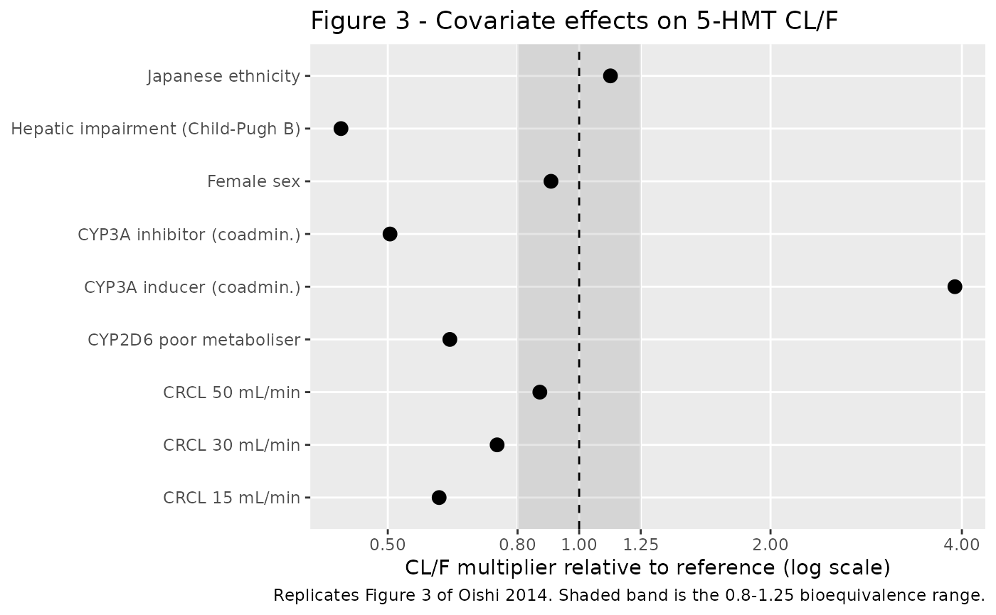
Replicate renal-impairment CL/F reductions from Discussion
The Discussion states that decreasing CRCL from 80 mL/min to 50, 30, and 15 mL/min gives 13.2%, 25.6%, and 39.5% decreases in CL/F, corresponding to 1.15-, 1.34-, and 1.65-fold increases in AUC.
crcl_vals <- c(80, 50, 30, 15)
crcl_ratio <- (crcl_vals / 80) ^ crcl_theta

renal_check <- data.frame(
  `CRCL (mL/min)`       = crcl_vals,
  `CL/F ratio vs. 80` = round(crcl_ratio, 3),
  `CL/F decrease (%)` = round(100 * (1 - crcl_ratio), 1),
  `AUC fold-change`   = round(1 / crcl_ratio, 2),
  check.names = FALSE
)

knitr::kable(
  renal_check,
  caption = "Renal-impairment CL/F reductions vs. reference (CRCL 80 mL/min). Compare with Oishi 2014 Discussion: 13.2% / 25.6% / 39.5% for CRCL 50 / 30 / 15."
)| CRCL (mL/min) | CL/F ratio vs. 80 | CL/F decrease (%) | AUC fold-change |
|---|---|---|---|
| 80 | 1.000 | 0.0 | 1.00 |
| 50 | 0.867 | 13.3 | 1.15 |
| 30 | 0.743 | 25.7 | 1.35 |
| 15 | 0.602 | 39.8 | 1.66 |
PKNCA validation
Non-compartmental analysis at steady state (day 7, single dosing interval 144 to 168 h) with treatment grouping by covariate arm.
sim_nca <- sim |>
  dplyr::filter(time >= 144, time <= 168, !is.na(Cc)) |>
  dplyr::mutate(time = time - 144) |>
  dplyr::select(id, time, Cc, arm)

# Guarantee a time-zero record for every (id, arm).
sim_nca <- dplyr::bind_rows(
  sim_nca,
  sim_nca |>
    dplyr::distinct(id, arm) |>
    dplyr::mutate(time = 0, Cc = 0)
) |>
  dplyr::distinct(id, arm, time, .keep_all = TRUE) |>
  dplyr::arrange(id, arm, time)

conc_obj <- PKNCA::PKNCAconc(sim_nca, Cc ~ time | arm + id)

dose_df <- arms |>
  dplyr::filter(evid == 1) |>
  dplyr::group_by(id, arm) |>
  dplyr::slice_max(time) |>
  dplyr::ungroup() |>
  dplyr::mutate(time = 0) |>
  dplyr::select(id, arm, time, amt)

dose_obj <- PKNCA::PKNCAdose(dose_df, amt ~ time | arm + id)

intervals <- data.frame(
  start   = 0,
  end     = 24,
  cmax    = TRUE,
  tmax    = TRUE,
  auclast = TRUE
)

nca_data <- PKNCA::PKNCAdata(conc_obj, dose_obj, intervals = intervals)
nca_res  <- PKNCA::pk.nca(nca_data)

nca_summary <- as.data.frame(nca_res) |>
  dplyr::group_by(arm, PPTESTCD) |>
  dplyr::summarise(median = median(PPORRES, na.rm = TRUE), .groups = "drop") |>
  tidyr::pivot_wider(names_from = PPTESTCD, values_from = median)

knitr::kable(
  nca_summary,
  digits = 3,
  caption = "Simulated steady-state NCA at 8 mg fesoterodine SR QD (day 7). Median across 200 subjects/arm."
)| arm | auclast | cmax | tmax |
|---|---|---|---|
| CYP2D6 poor metaboliser | 131.981 | 9.030 | 5.0 |
| CYP3A4 inducer (rifampicin) | 22.868 | 2.050 | 2.0 |
| CYP3A4 inhibitor (ketoconazole) | 176.255 | 11.872 | 5.5 |
| Hepatic impairment (Child-Pugh B) | 192.546 | 12.374 | 6.0 |
| Reference (EM Western male, CRCL 80) | 90.607 | 6.739 | 4.0 |
| Renal impairment (CRCL 15) | 135.879 | 9.228 | 5.0 |
The paper does not tabulate absolute Cmax / AUC values for the pooled population, so no direct side-by-side NCA comparison against the paper is provided here. The renal-impairment CL/F table above and the Figure 3 replicate together cover the paper’s principal quantitative claims about the final model.
Assumptions and deviations
-
Molecular-weight adjustment for CL/F and V/F. Oishi
2014 Methods ‘Data Analysis’ states that CL/F and V/F were adjusted by
the molecular weights of fesoterodine fumarate (527.65 g/mol) and 5-HMT
(341.5 g/mol) so that the administered fumarate dose reproduces the
5-HMT concentration when substituted directly into the model. This
vignette follows the paper’s convention:
amt = <dose_in_mg_fesoterodine_fumarate>is passed to the depot compartment, no explicit F-ratio is applied, and the model reproduces 5-HMT concentrations in ng/mL after the internal 1000x mg/L to ng/mL scaling on the observation variable. -
CRCL units. Oishi 2014 derived CRCL from the
Cockcroft-Gault equation, which returns mL/min (not BSA-normalised). The
canonical
CRCLcolumn accepts both BSA-normalised and raw Cockcroft-Gault values; per-model units are documented in the model file’scovariateData$CRCL$notes. Precedent: Delattre 2010 amikacin (raw Cockcroft-Gault). The reference value in the final equation is 80 mL/min in the same raw Cockcroft-Gault units. -
Reference-subject baseline (all binary indicators =
0). The model’s reference typical subject is a CYP2D6 EM
Western male, CRCL 80 mL/min, no concomitant CYP3A inhibitor or inducer,
and no hepatic impairment. Females and Japanese are represented by the
binary indicators
SEXFandRACE_JAPANESErespectively; Korean, other-Asian, and Westerner subjects all haveRACE_JAPANESE = 0. -
Tlag has no inter-individual variability. Oishi
2014 fixed the IIV on Tlag to zero because it could not be estimated
simultaneously with the ka IIV; the packaged model preserves this
decision by declaring no eta on
ltlag. - Preliminary 2-compartment model was rejected by the paper. Oishi 2014 Results state that a 2-compartment model with first-order absorption fit the Phase 1 data adequately but was unstable when the Phase 2/3 sparse- sampling data were added. The packaged model reproduces the paper’s final 1-compartment structural choice, not the preliminary 2-compartment form.
-
Study #10 and #13 CYP2D6 assignment. The paper’s
Methods ‘Covariate Model’ explains that subjects in studies #10
(Japanese single-dose healthy male) and #13 (Phase 2 Asian OAB) were not
genotyped for CYP2D6 and were classified as EM based on the ~1-2% PM
frequency reported in East Asian populations. The model’s
CYP2D6_PM = 0for these subjects mirrors that classification; the residual misclassification uncertainty is not carried through in the packaged model. -
Sex and Japanese ethnicity effects were retained despite
being clinically not-significant. Oishi 2014 Discussion notes
that the sex (0.903x) and Japanese (1.12x) multiplicative factors were
selected by the covariate search but the bootstrap 90% CIs both fell
within the 0.8-1.25 bioequivalence range; the authors concluded these
effects were not clinically significant. The packaged model retains them
so a downstream user can zero out either factor by setting
SEXForRACE_JAPANESEto zero at simulation time. - No source-paper NCA table for direct side-by-side comparison. The paper reports only the fitted CL/F ratios and CL/F reduction percentages (from the Discussion, transcribed above in the renal-impairment table); absolute Cmax / AUC values are not tabulated for the pooled population. The packaged validation therefore focuses on reproducing the paper’s covariate- effect claims rather than absolute exposure targets.