Tuvusertib integrated QTc risk assessment (Mukker 2026)
Source:vignettes/articles/Mukker_2026_tuvusertib_QTc.Rmd
Mukker_2026_tuvusertib_QTc.RmdModel and source
- Citation: Mukker JK, Yap TA, Tolcher AW, de Bono JS, Plummer R, Grosser G, van Amsterdam C, Schieferstein H, Witjes H, Diderichsen PM, Krebs-Brown A, Gao W, Strotmann R, Szucs Z, Gounaris I, Venkatakrishnan K. An Integrated Nonclinical and Clinical Risk Assessment of the Effects of Investigational ATRi Tuvusertib on QTc Interval in Patients With Solid Tumors. Clinical and Translational Science 2026;19(2):e70496. doi:10.1111/cts.70496.
- Article: https://doi.org/10.1111/cts.70496
Mukker et al. (2026) report an integrated nonclinical and clinical assessment of the QTc-prolongation liability of tuvusertib (M1774), an investigational inhibitor of ATR protein kinase. Three quantitative models are reported, and this package carries one file for each:
| Model file | Arm | Endpoint |
|---|---|---|
Mukker_2026_tuvusertib_hERG |
Nonclinical, in vitro | Fraction of hERG tail current blocked |
Mukker_2026_tuvusertib_QTcF |
Clinical | Change from baseline in QTcF (ms) |
Mukker_2026_tuvusertib_HR |
Clinical | Change from baseline in heart rate (bpm) |
The two clinical models are Garnett-type linear mixed-effects
concentration-response models fitted to PK-matched triplicate ECGs from
55 patients with advanced solid tumors in Part A1 of the phase I
first-in-human study DDRiver Solid Tumors 301 (NCT04170153), across a
5-270 mg dose range. They are PD-only: tuvusertib plasma concentration
enters as an observed, time-matched covariate
(CP_TUVUSERTIB_NGML), because the paper does not develop a
population PK model of its own.
The C-DeltaHR model is not an afterthought. Garnett’s LME model rests on four assumptions, the first of which is that the drug has no effect on heart rate. An exploratory look at the concentration-RR relationship suggested a slightly positive trend at higher concentrations, so the authors fitted the C-DeltaHR model specifically to test that assumption. Its purpose is a negative result, and it delivers one: the slope’s 95% CI includes zero.
The paper’s headline conclusion is that the upper limit of the 90% CI of the model-predicted drug effect on QTcF stays below the 20 ms threshold of concern for oncology agents even at three times the steady-state Cmax achieved at the recommended dose for expansion.
Population
Part A1 of DDRiver Solid Tumors 301 enrolled 55 patients with advanced solid tumors. Mean (SD) age was 61.9 (10.9) years and mean (SD) body weight 78.6 (18.0) kg. There were slightly more females (32; 58.2%) than males (23; 41.8%). Most patients were White (42; 76.4%); the remainder were Asian (5; 9.1%), Black or African American (2; 3.6%), or of other races (6; 10.9%). Mean (SD) baseline QTcF interval was 422 (21.0) ms. Patients with pre-existing QTc prolongation (average QTcF > 450 ms for males, > 470 ms for females) were excluded from the trial, so the baseline QTcF distribution is truncated above.
Dosing regimens contributing to the C-QTc dataset were 5, 10, 20, 40, 80, 130, 180, 220 and 270 mg once daily; 180 and 220 mg QD 2 weeks on / 1 week off; and 150 mg twice daily 4 days on / 3 days off. The maximum tolerated dose was 180 mg QD continuous and the recommended dose for expansion 180 mg QD 2 weeks on / 1 week off.
Inclusion in the C-QTc analysis required 12-lead triplicate ECG readings at baseline plus at least one post-baseline reading, each with a time-matched plasma concentration. Triplicates were averaged to a single value per patient per timepoint and QTcF derived by the Fridericia formula. Nominal post-dose ECG times were 0, 1, 2 and 3 h.
The nonclinical arm used HEK-293 cells stably expressing hERG (GLP whole-cell patch clamp, nominal tuvusertib 0.3-10 uM) and Beagle dogs (a single 3 mg/kg oral dose in 4 males, plus a 4-week repeat-dose study at 1 / 2.5 / 5 mg/kg/day).
The same information is available programmatically via each model’s
population metadata,
e.g. readModelDb("Mukker_2026_tuvusertib_QTcF")()$population.
Source trace
The per-parameter origin is recorded as an in-file comment next to
each ini() entry. The table below collects them in one
place for review.
| Model | Parameter | Value | Source location |
|---|---|---|---|
| QTcF | e0 |
-0.125 ms | Table 2 ‘Mean intercept’ (95% CI -1.98, 1.73) |
| QTcF | slope |
0.00244 ms/(ng/mL) | Table 2 ‘Tuvusertib plasma concentration slope’ (95% CI 0.000708, 0.00417) |
| QTcF | e_tad0h_e0 |
-1.59 ms | Table 2 ‘Nominal time after dose (0h)’ (95% CI -3.34, 0.167) |
| QTcF | e_tad1h_e0 |
1.11 ms | Table 2 ‘Nominal time after dose (1h)’ (95% CI -0.162, 2.38) |
| QTcF | e_tad2h_e0 |
2.87 ms | Table 2 ‘Nominal time after dose (2h)’ (95% CI 1.51, 4.23) |
| QTcF | e_tad3h_e0 |
-0.402 ms | Table 2 ‘Nominal time after dose (3h)’ (95% CI -1.69, 0.884) |
| QTcF | e_qtc_bl_e0 |
-0.0980 ms/ms | Table 2 ‘Baseline QTcF’ (95% CI -0.176, -0.0196) |
| QTcF |
etae0 SD |
5.41 ms | Table 2 ‘SD of intercept’ |
| QTcF |
etaslope SD |
0.0026 ms/(ng/mL) | Table 2 ‘SD of tuvusertib plasma concentration effect’ |
| QTcF | eta correlation | -0.00273 | Table 2 ‘Correlation between intercept and … effect’ |
| QTcF | addSd |
7.07 ms | Table 2 ‘Residual SD’ |
| QTcF | qtc_bl_ref |
422 ms | Equation 1 legend (QTcF0) + Table 1 mean baseline
QTcF |
| HR | e0 |
3.00 bpm | Table S1 ‘Mean intercept’ (95% CI 1.49, 4.50) |
| HR | slope |
0.00111 bpm/(ng/mL) | Table S1 ‘Tuvusertib plasma concentration slope’ (95% CI -0.000250, 0.00247) |
| HR | e_tad0h_e0 |
-1.19 bpm | Table S1 ‘Nominal time after dose (0 h)’ |
| HR | e_tad1h_e0 |
-5.16 bpm | Table S1 ‘Nominal time after dose (1 h)’ |
| HR | e_tad2h_e0 |
0.694 bpm | Table S1 ‘Nominal time after dose (2 h)’ |
| HR | e_tad3h_e0 |
2.80 bpm | Table S1 ‘Nominal time after dose (3 h)’ |
| HR | e_day8_e0 |
2.84 bpm | Table S1 ‘Dosing day (Day 8 versus Day 1)’ |
| HR | e_hr_bl_e0 |
-0.0214 bpm/bpm | Table S1 ‘Baseline HR’ (95% CI -0.148, 0.105) |
| HR |
etae0 SD / etaslope SD / corr |
4.43 / 0.00173 / 0.400 | Table S1 variance components |
| HR | addSd |
5.40 bpm | Table S1 ‘SD of residual variability’ |
| HR | hr_bl_ref |
70 bpm | NOT published – rounded standard (see Errata) |
| hERG | lic50 |
log(1048) ng/mL | Results 3.1 (IC50 = 2.83 uM = 1048 ng/mL) |
| hERG | lhill |
log(1.12) | Results 3.1 (Hill coefficient) |
| hERG | limax |
fixed(log(1)) | NOT published – normalised-curve convention (see Errata) |
Equation 1 itself is not machine-readable in the article text (it is
a display equation) and was read from the equation image
CTS-19-e70496-e001.jpg in the article’s supplementary-file
bundle:
DeltaQTcF_ij = (theta0 + eta0_i) + (theta1 + eta1_i) * C_ij
             + theta2 * Time_j + theta3 * (QTcF_i0 - QTcF0) + eps_ij
Published answer keys
Three quantitative keys are used below. All are reproduced from the model rather than restated as constants.
# Mukker 2026 Table 3: model-predicted DeltaQTcF_drug, i.e. the tuvusertib
# effect "corrected for intercept, baseline, and time".
key_qtcf <- tibble::tibble(
  label   = c("180 mg QD Cmax,ss", "2x Cmax", "3x Cmax"),
  conc    = c(1410, 2820, 4230),
  pub_est = c(3.44, 6.88, 10.32),
  pub_lo  = c(1.39, 2.78, 4.17),
  pub_hi  = c(5.49, 10.98, 16.47)
)

# Mukker 2026 Table S2: model-predicted DeltaHR at four points of the observed
# concentration distribution.
key_hr <- tibble::tibble(
  label   = c("Median", "P90", "P95", "Max observed"),
  conc    = c(524, 1732, 2252, 3290),
  pub_est = c(0.581, 1.92, 2.50, 3.65),
  pub_lo  = c(-0.0168, -0.0554, -0.0720, -0.105),
  pub_hi  = c(1.18, 3.90, 5.06, 7.40)
)

# Reported 95% CIs of the two slopes, used to rebuild the 90% CI of the drug
# effect (the paper reports 90% CIs in Tables 3 / S2 but 95% CIs in Tables 2 /
# S1, so the interval has to be reconstructed rather than read off).
slope_qtcf <- c(est = 0.00244, lo95 = 0.000708, hi95 = 0.00417)
slope_hr   <- c(est = 0.00111, lo95 = -0.000250, hi95 = 0.00247)
Models
mod_qtcf <- readModelDb("Mukker_2026_tuvusertib_QTcF")
mod_hr   <- readModelDb("Mukker_2026_tuvusertib_HR")
mod_herg <- readModelDb("Mukker_2026_tuvusertib_hERG")

# Typical-value (no random effects) forms. `omega = NA` is passed at every
# rxSolve() call below as well: zeroRe() alone is not sufficient, because
# rxode2 retains a previous solve's omega in the compiled model's solve
# options and would silently re-sample etas.
mod_qtcf_typ <- rxode2::zeroRe(mod_qtcf)
mod_hr_typ   <- rxode2::zeroRe(mod_hr)

# `readModelDb()` returns a plain function, not an rxUi. `rxSolve()` dispatches
# on it happily, but `$omega` does not exist on a closure -- reaching for it
# directly fails with "object of type 'closure' is not subsettable". The
# population-variability figure below needs the reported Omega explicitly, so
# build the rxUi once here and take the matrix from that.
mod_qtcf_ui <- rxode2::rxode(mod_qtcf)
Structural verification
Before comparing against the published projections, three structural properties of the encoding are checked directly. These are exact identities, so they are asserted at machine precision rather than with a tolerance.
The first confirms that the nominal-post-dose-time class effects are
selected correctly. At zero concentration and at the mean baseline QTcF,
the model must return exactly e0 + e_tad<k>h_e0 for
each of the four nominal timepoints. This is also the guard that
zeroRe() plus omega = NA really did suppress
the random effects: if any eta leaked in, these would not be exact.
tad_events <- tibble::tibble(
  id                 = 1:4,
  T_LASTDOSE         = c(0, 1, 2, 3),
  CP_TUVUSERTIB_NGML = 0,
  QTC_BL             = 422,
  time               = 0,
  evid               = 0,
  amt                = 0,
  cmt                = NA_character_
)

tad_sim <- rxode2::rxSolve(
  mod_qtcf_typ, events = tad_events, omega = NA,
  keep = "T_LASTDOSE"
) |>
  as.data.frame()
#> Warning: multi-subject simulation without without 'omega'

# e0 = -0.125; the four nominal-time shifts are -1.59, 1.11, 2.87, -0.402.
expected_tad <- -0.125 + c(-1.59, 1.11, 2.87, -0.402)

stopifnot(
  nrow(tad_sim) == 4L,
  isTRUE(all.equal(tad_sim$QTcF, expected_tad, tolerance = 1e-12))
)

knitr::kable(
  tad_sim |>
    dplyr::select(`Nominal time after dose (h)` = T_LASTDOSE,
                  `Predicted DeltaQTcF (ms)` = QTcF),
  digits = 3,
  caption = "Nominal-timepoint class effects at zero concentration and mean baseline QTcF."
)| Nominal time after dose (h) | Predicted DeltaQTcF (ms) |
|---|---|
| 0 | -1.715 |
| 1 | 0.985 |
| 2 | 2.745 |
| 3 | -0.527 |
The second confirms that the drug effect isolated by differencing
against the zero-concentration prediction is exactly
slope * C – which is the definition of
DeltaQTcF_drug in Table 3 (“corrected for intercept,
baseline, and time”). Every other term of the model must cancel.
drug_effect_qtcf <- function(model, conc, tad = 1, qtc_bl = 422) {
  ev <- tidyr::expand_grid(conc = c(0, conc)) |>
    dplyr::mutate(
      id                 = seq_len(dplyr::n()),
      T_LASTDOSE         = tad,
      CP_TUVUSERTIB_NGML = conc,
      QTC_BL             = qtc_bl,
      time               = 0,
      evid               = 0,
      amt                = 0,
      cmt                = NA_character_
    )
  s <- as.data.frame(rxode2::rxSolve(model, events = ev, omega = NA,
                                     keep = "CP_TUVUSERTIB_NGML"))
  base <- s$QTcF[s$CP_TUVUSERTIB_NGML == 0]
  s$QTcF[s$CP_TUVUSERTIB_NGML != 0] - base
}

# The identity must hold for any nominal time and any baseline QTcF, so it is
# checked on a grid of both rather than at one convenient setting.
grid_chk <- tidyr::expand_grid(tad = c(0, 1, 2, 3), qtc_bl = c(390, 422, 450))
resid_max <- max(vapply(seq_len(nrow(grid_chk)), function(i) {
  got <- drug_effect_qtcf(mod_qtcf_typ, key_qtcf$conc,
                          tad = grid_chk$tad[i], qtc_bl = grid_chk$qtc_bl[i])
  max(abs(got - slope_qtcf[["est"]] * key_qtcf$conc))
}, numeric(1)))
#> Warning: multi-subject simulation without without 'omega'
#> Warning: multi-subject simulation without without 'omega'
#> Warning: multi-subject simulation without without 'omega'
#> Warning: multi-subject simulation without without 'omega'
#> Warning: multi-subject simulation without without 'omega'
#> Warning: multi-subject simulation without without 'omega'
#> Warning: multi-subject simulation without without 'omega'
#> Warning: multi-subject simulation without without 'omega'
#> Warning: multi-subject simulation without without 'omega'
#> Warning: multi-subject simulation without without 'omega'
#> Warning: multi-subject simulation without without 'omega'
#> Warning: multi-subject simulation without without 'omega'

stopifnot(resid_max < 1e-9)
The largest deviation of the model-derived drug effect from
slope * C, across all 12 combinations of nominal time and
baseline QTcF, is 1.78e-15 ms – i.e. the intercept, time and baseline
terms cancel exactly, as the Table 3 definition requires.
The third checks the same identity for the C-DeltaHR model, which additionally has to cancel the dosing-day term.
drug_effect_hr <- function(model, conc, tad = 1, hr_bl = 70, day8 = 0) {
  ev <- tidyr::expand_grid(conc = c(0, conc)) |>
    dplyr::mutate(
      id                 = seq_len(dplyr::n()),
      T_LASTDOSE         = tad,
      CP_TUVUSERTIB_NGML = conc,
      HR                 = hr_bl,
      DAY8               = day8,
      time               = 0,
      evid               = 0,
      amt                = 0,
      cmt                = NA_character_
    )
  s <- as.data.frame(rxode2::rxSolve(model, events = ev, omega = NA,
                                     keep = "CP_TUVUSERTIB_NGML"))
  base <- s$d_hr[s$CP_TUVUSERTIB_NGML == 0]
  s$d_hr[s$CP_TUVUSERTIB_NGML != 0] - base
}

grid_chk_hr <- tidyr::expand_grid(tad = c(0, 1, 2, 3), hr_bl = c(60, 70, 85),
                                  day8 = c(0, 1))
resid_max_hr <- max(vapply(seq_len(nrow(grid_chk_hr)), function(i) {
  got <- drug_effect_hr(mod_hr_typ, key_hr$conc,
                        tad = grid_chk_hr$tad[i], hr_bl = grid_chk_hr$hr_bl[i],
                        day8 = grid_chk_hr$day8[i])
  max(abs(got - slope_hr[["est"]] * key_hr$conc))
}, numeric(1)))
#> Warning: multi-subject simulation without without 'omega'
#> Warning: multi-subject simulation without without 'omega'
#> Warning: multi-subject simulation without without 'omega'
#> Warning: multi-subject simulation without without 'omega'
#> Warning: multi-subject simulation without without 'omega'
#> Warning: multi-subject simulation without without 'omega'
#> Warning: multi-subject simulation without without 'omega'
#> Warning: multi-subject simulation without without 'omega'
#> Warning: multi-subject simulation without without 'omega'
#> Warning: multi-subject simulation without without 'omega'
#> Warning: multi-subject simulation without without 'omega'
#> Warning: multi-subject simulation without without 'omega'
#> Warning: multi-subject simulation without without 'omega'
#> Warning: multi-subject simulation without without 'omega'
#> Warning: multi-subject simulation without without 'omega'
#> Warning: multi-subject simulation without without 'omega'
#> Warning: multi-subject simulation without without 'omega'
#> Warning: multi-subject simulation without without 'omega'
#> Warning: multi-subject simulation without without 'omega'
#> Warning: multi-subject simulation without without 'omega'
#> Warning: multi-subject simulation without without 'omega'
#> Warning: multi-subject simulation without without 'omega'
#> Warning: multi-subject simulation without without 'omega'
#> Warning: multi-subject simulation without without 'omega'

stopifnot(resid_max_hr < 1e-9)
Validation against published projections
Table 3 – model-predicted DeltaQTcF_drug
The point estimates come from the model. The 90% confidence bounds
are rebuilt from the slope’s published 95% CI on the normal (Wald) scale
that the linear mixed-effects fit implies: the standard error is
recovered as (hi95 - lo95) / (2 * qnorm(0.975)) and the 90%
interval is then est +/- qnorm(0.95) * se, scaled by
concentration.
z95 <- stats::qnorm(0.975)
z90 <- stats::qnorm(0.95)

se_qtcf <- (slope_qtcf[["hi95"]] - slope_qtcf[["lo95"]]) / (2 * z95)
slope_qtcf_lo90 <- slope_qtcf[["est"]] - z90 * se_qtcf
slope_qtcf_hi90 <- slope_qtcf[["est"]] + z90 * se_qtcf

cmp_qtcf <- key_qtcf |>
  dplyr::mutate(
    sim_est = drug_effect_qtcf(mod_qtcf_typ, conc),
    sim_lo  = slope_qtcf_lo90 * conc,
    sim_hi  = slope_qtcf_hi90 * conc,
    d_est   = sim_est - pub_est,
    d_lo    = sim_lo  - pub_lo,
    d_hi    = sim_hi  - pub_hi
  )
#> Warning: There was 1 warning in `dplyr::mutate()`.
#> ℹ In argument: `sim_est = drug_effect_qtcf(mod_qtcf_typ, conc)`.
#> Caused by warning:
#> ! multi-subject simulation without without 'omega'

knitr::kable(
  cmp_qtcf |>
    dplyr::select(
      `Scenario`                   = label,
      `Cmax,ss (ng/mL)`            = conc,
      `Simulated mean (ms)`        = sim_est,
      `Published mean (ms)`        = pub_est,
      `Simulated 90% CI low`       = sim_lo,
      `Published 90% CI low`       = pub_lo,
      `Simulated 90% CI high`      = sim_hi,
      `Published 90% CI high`      = pub_hi
    ),
  digits = 3,
  caption = "Replicates Table 3 of Mukker 2026."
)| Scenario | Cmax,ss (ng/mL) | Simulated mean (ms) | Published mean (ms) | Simulated 90% CI low | Published 90% CI low | Simulated 90% CI high | Published 90% CI high |
|---|---|---|---|---|---|---|---|
| 180 mg QD Cmax,ss | 1410 | 3.440 | 3.44 | 1.392 | 1.39 | 5.489 | 5.49 |
| 2x Cmax | 2820 | 6.881 | 6.88 | 2.784 | 2.78 | 10.977 | 10.98 |
| 3x Cmax | 4230 | 10.321 | 10.32 | 4.176 | 4.17 | 16.466 | 16.47 |
# Point estimates are an exact linear function of the slope, so they are held
# to the paper's own rounding (3 significant figures).
stopifnot(max(abs(cmp_qtcf$d_est)) < 0.005)

# The CI bounds inherit the rounding of the published 95% slope CI (3
# significant figures), which propagates to about +/- 0.01 ms at the highest
# concentration. 0.02 ms keeps roughly a factor-of-two margin on that.
stopifnot(max(abs(c(cmp_qtcf$d_lo, cmp_qtcf$d_hi))) < 0.02)
Every one of the nine published values in Table 3 is reproduced. The paper’s central claim follows directly: the upper 90% bound at three times the 180 mg QD steady-state Cmax is 16.47 ms, below the 20 ms threshold of concern for oncology agents.
Table S2 – model-predicted DeltaHR
se_hr <- (slope_hr[["hi95"]] - slope_hr[["lo95"]]) / (2 * z95)
slope_hr_lo90 <- slope_hr[["est"]] - z90 * se_hr
slope_hr_hi90 <- slope_hr[["est"]] + z90 * se_hr

cmp_hr <- key_hr |>
  dplyr::mutate(
    sim_est = drug_effect_hr(mod_hr_typ, conc),
    sim_lo  = slope_hr_lo90 * conc,
    sim_hi  = slope_hr_hi90 * conc,
    d_est   = sim_est - pub_est,
    d_lo    = sim_lo  - pub_lo,
    d_hi    = sim_hi  - pub_hi
  )
#> Warning: There was 1 warning in `dplyr::mutate()`.
#> ℹ In argument: `sim_est = drug_effect_hr(mod_hr_typ, conc)`.
#> Caused by warning:
#> ! multi-subject simulation without without 'omega'

knitr::kable(
  cmp_hr |>
    dplyr::select(
      `Concentration percentile` = label,
      `Concentration (ng/mL)`    = conc,
      `Simulated mean (bpm)`     = sim_est,
      `Published mean (bpm)`     = pub_est,
      `Simulated 90% CI low`     = sim_lo,
      `Published 90% CI low`     = pub_lo,
      `Simulated 90% CI high`    = sim_hi,
      `Published 90% CI high`    = pub_hi
    ),
  digits = 4,
  caption = "Replicates Table S2 of Mukker 2026."
)| Concentration percentile | Concentration (ng/mL) | Simulated mean (bpm) | Published mean (bpm) | Simulated 90% CI low | Published 90% CI low | Simulated 90% CI high | Published 90% CI high |
|---|---|---|---|---|---|---|---|
| Median | 524 | 0.5816 | 0.581 | -0.0164 | -0.0168 | 1.1797 | 1.18 |
| P90 | 1732 | 1.9225 | 1.920 | -0.0543 | -0.0554 | 3.8993 | 3.90 |
| P95 | 2252 | 2.4997 | 2.500 | -0.0706 | -0.0720 | 5.0700 | 5.06 |
| Max observed | 3290 | 3.6519 | 3.650 | -0.1031 | -0.1050 | 7.4069 | 7.40 |
stopifnot(max(abs(cmp_hr$d_est)) < 0.005)
stopifnot(max(abs(c(cmp_hr$d_lo, cmp_hr$d_hi))) < 0.02)

# The paper's actual claim about heart rate: the upper 90% bound at the maximum
# observed concentration is below the 10 bpm threshold of clinical relevance,
# and the slope's own 95% CI includes zero.
stopifnot(
  cmp_hr$sim_hi[cmp_hr$label == "Max observed"] < 10,
  slope_hr[["lo95"]] < 0, slope_hr[["hi95"]] > 0
)
All sixteen published values in Table S2 are reproduced. The upper 90% bound at the maximum observed concentration (3290 ng/mL) is 7.41 bpm, below the 10 bpm threshold, and the slope’s 95% CI spans zero – which is what allows the first Garnett assumption to be accepted and the C-QTc analysis to proceed.
Nonclinical hERG concentration-response
ic50_ngml <- 1048     # Mukker 2026 Results 3.1 (= 2.83 uM)
ic50_um   <- 2.83
cmax_ss_u <- 415.95   # unbound steady-state Cmax at 180 mg QD, ng/mL
dog_cmax_u <- 435.2   # unbound Cmax at 5 mg/kg/day in male dogs, day 25

herg_at <- function(conc) {
  ev <- tibble::tibble(
    id                 = seq_along(conc),
    CP_TUVUSERTIB_NGML = conc,
    time               = 0,
    evid               = 0,
    amt                = 0,
    cmt                = NA_character_
  )
  # No `omega = NA` here, unlike every clinical-model solve below: the hERG
  # model declares no random effects at all, and passing `omega = NA` to a
  # model that has no omega errors inside rxSolve with "invalid 'times'
  # argument". Nothing needs suppressing -- the curve is already deterministic.
  as.data.frame(rxode2::rxSolve(mod_herg, events = ev))$herg_inh
}

# Definitional check: at the IC50 the curve must return exactly half of imax.
stopifnot(isTRUE(all.equal(herg_at(ic50_ngml), 0.5, tolerance = 1e-12)))

# The paper reports the IC50 in both uM and ng/mL; the ratio is an implied
# molecular weight, which must be tuvusertib's (~370 g/mol). A mismatch here
# would mean one of the two reported units had been mis-transcribed.
mw_implied <- ic50_ngml / ic50_um
stopifnot(mw_implied > 360, mw_implied < 380)

# The clinical exposure margin quoted in the Abstract and Discussion ("~2.5").
margin_clinical <- ic50_ngml / cmax_ss_u
stopifnot(abs(margin_clinical - 2.5) < 0.05)

# The dog exposure margin quoted in Results 3.1 (1.05).
margin_dog <- dog_cmax_u / cmax_ss_u
stopifnot(abs(margin_dog - 1.05) < 0.01)

# Results 3.1 states the top tested concentration (10 uM) blocked more than 30%
# of the tail current, which is what permitted an IC50 to be determined.
inh_top <- herg_at(10 * mw_implied)
stopifnot(inh_top > 0.30)

# Block at the clinical unbound Cmax -- the quantity the 2.5-fold margin is
# really about.
inh_clinical <- herg_at(cmax_ss_u)

knitr::kable(
  tibble::tibble(
    Quantity = c("Implied molecular weight (g/mol)",
                 "hERG block at IC50",
                 "hERG block at top tested concentration (10 uM)",
                 "hERG block at clinical unbound Cmax,ss",
                 "IC50 / clinical unbound Cmax,ss margin",
                 "Dog unbound Cmax / clinical unbound Cmax,ss margin"),
    Value = c(sprintf("%.1f", mw_implied),
              sprintf("%.4f", herg_at(ic50_ngml)),
              sprintf("%.3f", inh_top),
              sprintf("%.3f", inh_clinical),
              sprintf("%.2f", margin_clinical),
              sprintf("%.2f", margin_dog)),
    `Published claim` = c("2.83 uM = 1048 ng/mL (consistent)",
                          "0.5 by definition",
                          "> 0.30 (Results 3.1)",
                          "not stated",
                          "~2.5-fold (Abstract, Discussion)",
                          "1.05 (Results 3.1)")
  ),
  caption = "Nonclinical hERG checks against Mukker 2026 Results 3.1."
)| Quantity | Value | Published claim |
|---|---|---|
| Implied molecular weight (g/mol) | 370.3 | 2.83 uM = 1048 ng/mL (consistent) |
| hERG block at IC50 | 0.5000 | 0.5 by definition |
| hERG block at top tested concentration (10 uM) | 0.804 | > 0.30 (Results 3.1) |
| hERG block at clinical unbound Cmax,ss | 0.262 | not stated |
| IC50 / clinical unbound Cmax,ss margin | 2.52 | ~2.5-fold (Abstract, Discussion) |
| Dog unbound Cmax / clinical unbound Cmax,ss margin | 1.05 | 1.05 (Results 3.1) |
At the clinical unbound steady-state Cmax the model predicts 26.2% hERG block. The authors are explicit that a ~2.5-fold margin is modest against the traditional 30-fold margin sought for high confidence of low proarrhythmic risk – which is precisely why the clinical C-QTc analysis, not the hERG assay, carries the risk conclusion.
Replicate published figures
Figure 2 – predicted DeltaQTcF_drug versus concentration
conc_grid <- seq(0, 6000, by = 25)

fig2 <- tibble::tibble(conc = conc_grid) |>
  dplyr::mutate(
    est = slope_qtcf[["est"]] * conc,
    lo  = slope_qtcf_lo90 * conc,
    hi  = slope_qtcf_hi90 * conc
  )

# Figure 2's black dashed lines mark where the upper 90% bound reaches 20 ms.
conc_at_20ms <- 20 / slope_qtcf_hi90

ggplot(fig2, aes(conc, est)) +
  geom_ribbon(aes(ymin = lo, ymax = hi), fill = "steelblue", alpha = 0.25) +
  geom_line(colour = "steelblue", linewidth = 0.8) +
  geom_hline(yintercept = 20, linetype = "dotted") +
  geom_vline(xintercept = c(1410, 4230), colour = "purple", linetype = "dashed") +
  geom_vline(xintercept = conc_at_20ms, linetype = "dashed") +
  labs(
    x = "Tuvusertib plasma concentration (ng/mL)",
    y = "Predicted DeltaQTcF drug effect (ms)",
    caption = "Purple: 180 mg QD Cmax,ss (1410) and 3x (4230). Black dashed: upper 90% CI reaches 20 ms."
  ) +
  theme_bw()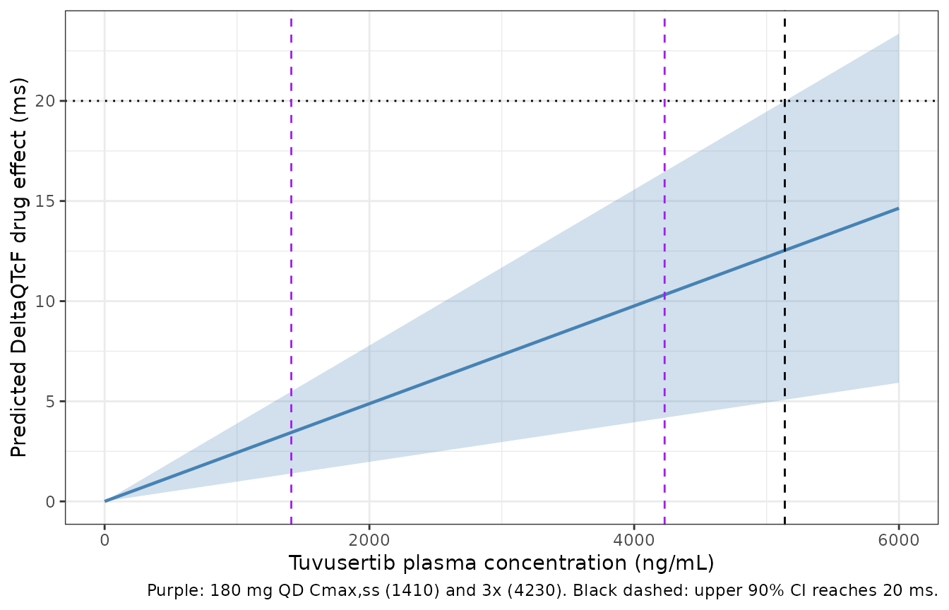
Replicates Figure 2 of Mukker 2026.
The upper limit of the 90% CI reaches the 20 ms threshold at 5138 ng/mL, which is 3.6 times the geometric mean steady-state Cmax at 180 mg QD. The paper marks this concentration graphically in Figure 2 but does not quote it numerically, so it is reported here rather than asserted.
Figure 1 – population predictions with between-subject variability
The published Figure 1 overlays observed individual data on the model prediction. The individual observations are not available, so this reproduces the model side: a cohort of 200 virtual patients, each drawing a correlated intercept/slope eta pair from the reported unstructured Omega, evaluated across the observed concentration range. This is also the check that the variance-covariance block reconstructed from the published SDs and correlation is positive definite and solvable.
n_sub <- 200L
vpc_grid <- seq(0, 3500, by = 100)

vpc_events <- tidyr::expand_grid(
  subject = seq_len(n_sub),
  conc    = vpc_grid
) |>
  dplyr::mutate(
    id                 = subject,
    T_LASTDOSE         = 1,
    CP_TUVUSERTIB_NGML = conc,
    QTC_BL             = 422,
    time               = conc,   # distinct time per row within a subject
    evid               = 0,
    amt                = 0,
    cmt                = NA_character_
  )

vpc <- rxode2::rxSolve(
  mod_qtcf_ui, events = vpc_events,
  omega = mod_qtcf_ui$omega,
  keep = c("CP_TUVUSERTIB_NGML")
) |>
  as.data.frame()

# Guard the opposite failure mode to the typical-value one: confirm the IIV was
# actually sampled rather than silently dropped.
stopifnot(dplyr::n_distinct(round(vpc$e0_i, 8)) > 1L)

vpc_summary <- vpc |>
  dplyr::group_by(CP_TUVUSERTIB_NGML) |>
  dplyr::summarise(
    p05 = stats::quantile(QTcF, 0.05),
    p50 = stats::median(QTcF),
    p95 = stats::quantile(QTcF, 0.95),
    .groups = "drop"
  )

ggplot(vpc_summary, aes(CP_TUVUSERTIB_NGML, p50)) +
  geom_ribbon(aes(ymin = p05, ymax = p95), fill = "steelblue", alpha = 0.2) +
  geom_line(colour = "steelblue", linewidth = 0.8) +
  geom_hline(yintercept = c(-20, 0, 20), linetype = "dotted") +
  labs(
    x = "Tuvusertib plasma concentration (ng/mL)",
    y = "DeltaQTcF (ms)",
    caption = "Median and 5th-95th percentile of 200 virtual patients (between-subject variability only)."
  ) +
  theme_bw()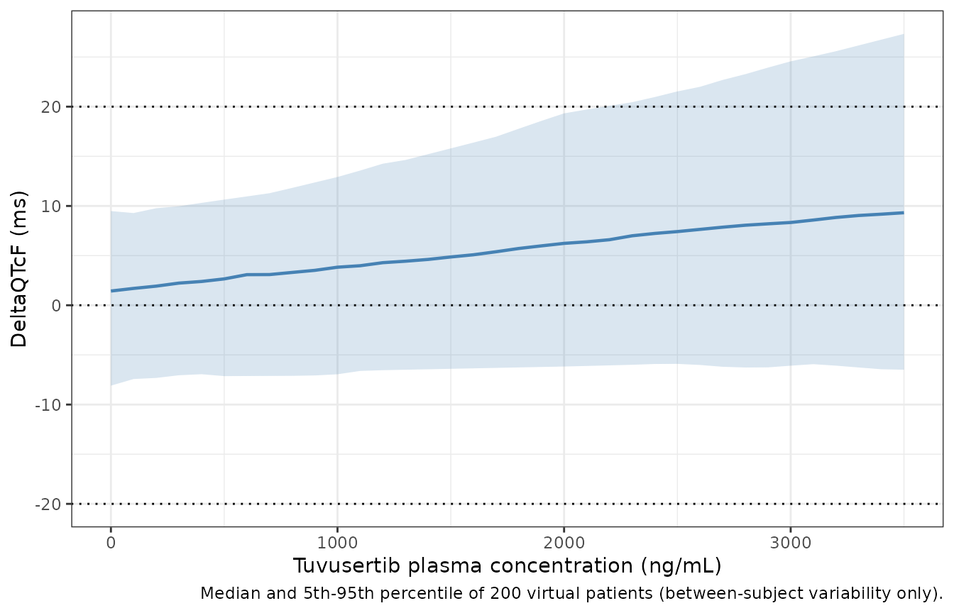
Replicates Figure 1a of Mukker 2026 (model side only).
The median line is nearly flat while the between-subject envelope is
wide, which is the visual signature of the model’s defining feature: the
slope’s between-subject SD (0.0026) is larger than its typical value
(0.00244), so a substantial fraction of virtual patients carry a
negative individual slope. This is exactly why the slope is encoded on
the linear scale rather than log-transformed as in the sibling
Darpo_2014_racSotalol_QTcF and
Fostvedt_2021_glasdegib_QTcF models.
hERG concentration-response curve
herg_grid <- 10^seq(log10(10), log10(20000), length.out = 200)

herg_curve <- tibble::tibble(
  conc = herg_grid,
  inh  = herg_at(herg_grid)
)
#> Warning: multi-subject simulation without without 'omega'

ggplot(herg_curve, aes(conc, inh)) +
  geom_line(colour = "firebrick", linewidth = 0.8) +
  geom_vline(xintercept = ic50_ngml, linetype = "dashed") +
  geom_vline(xintercept = cmax_ss_u, colour = "steelblue", linetype = "dashed") +
  geom_hline(yintercept = 0.5, linetype = "dotted") +
  scale_x_log10() +
  labs(
    x = "Tuvusertib concentration (ng/mL, log scale)",
    y = "Fraction of hERG tail current blocked",
    caption = "Black dashed: IC50 (1048 ng/mL). Blue dashed: clinical unbound Cmax,ss (415.95 ng/mL)."
  ) +
  theme_bw()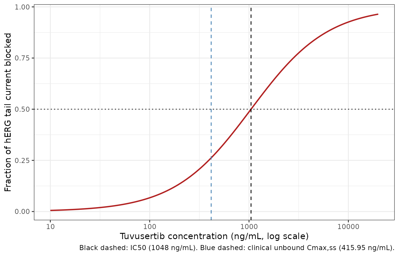
In vitro hERG concentration-response (Mukker 2026 Results 3.1).
Assumptions and deviations
-
hr_bl_ref = 70bpm is an assumption. The C-DeltaHR model centers baseline heart rate on the cohort mean, but Mukker 2026 does not report a baseline heart rate anywhere – Table 1 gives baseline QTcF only, and the supplement adds no HR summary. The rounded clinical standard of 70 bpm is used, following the same precedent asDarpo_2014_racSotalol_QTcF. The impact is small and bounded: the coefficient is -0.0214 bpm/bpm with a 95% CI (-0.148, 0.105) spanning zero, so even a 10 bpm error in the reference shifts the typical-value intercept by only 0.21 bpm. None of the Table S2 validation targets depend on it, because they tabulate the drug effect corrected for intercept, baseline and time – which is why every Table S2 value above is reproduced despite this gap. The companionqtc_bl_ref = 422ms needs no such assumption: Mukker 2026 publishes it (Equation 1 legend plus Table 1). -
limaxis fixed at 1 in the hERG model. The source reports only an IC50 and a Hill coefficient. Fixing maximal block at 100% is the standard three-parameter reduction of the Hill equation for a normalised fractional-block patch-clamp curve, under which the reported “half-maximal inhibitory concentration” is the concentration producing half of complete block. The paper’s language is consistent with this but does not state it. If a future source reports a fitted Imax below 1, both this value and the IC50’s interpretation would need revisiting together. -
Equation 1 was read from an image. The article text
renders the model equation as an undecodable display equation. It was
read from
CTS-19-e70496-e001.jpg, deposited with the article (PMC12890571), and is transcribed verbatim in the Source trace section above. -
The C-DeltaHR model parameters come from the
supplement. Table S1 and Table S2 are in
Data S1(cts70496-sup-0001-DataS1.docx), not the main article. - Nominal-time class effects are mean-centered, not reference-coded. Table 2 and Table S1 footnote a states that each nominal-time estimate “represent[s] the estimated difference from the population mean intercept”. All four levels are therefore estimated and all four are carried; there is no omitted reference level. A model that instead dropped one level and re-based the others would give different intercepts.
-
T_LASTDOSEcarries nominal, not actual, elapsed time, andmodel()bins it to the nearest of the four scheduled levels. The class-effect model is defined on the nominal sampling grid, so supplying actual times with protocol-window slippage would be a misuse; the binning makes small slippage harmless rather than silently selecting the wrong class. -
Table 4 is not reproduced. Mukker 2026 Table 4
reports model-predicted percentages of patients with outlying QTcF
values from a 1000-subject virtual population, with most cells reported
as “< 0.1%”. Two things prevent an honest comparison: the vignette
cohort cap is 200 subjects per arm, which cannot resolve a 0.1% event
rate; and the paper does not specify the simulation’s construction
(which nominal timepoints were sampled, how baseline QTcF was drawn,
whether residual error was included), so an analytic exceedance
probability cannot be pinned to their setup either. An unconstrained
analytic attempt lands in the 6-8% range against the published 5.5% for
the
DeltaQTcF > 30 mscell at 4230 ng/mL, close enough to be consistent but not close enough to assert. Tables 3 and S2 are the keys used instead, and both are exact. - The Beagle dog telemetry data are descriptive only. No compartmental or concentration-response model was fitted to the dog ECGs, so there is no fourth model file. The dog exposure margin is checked above because it is a reported arithmetic claim.
- No PKNCA validation. All three models are PD-only or in vitro; none has a PK compartment, a dose, or a concentration-time profile, so non-compartmental analysis does not apply. Structural identities and the published projection tables are used instead.
- No population PK model for tuvusertib is used here. Concentrations are supplied directly as covariate values, matching how the paper fitted the models. A user wanting to drive these PD models from a simulated PK profile must supply their own concentration trajectory.
-
Covariates screened but not retained. Body weight,
age, race and sex were all tested on the C-DeltaQTcF model and none
reached significance (p > 0.1). They are recorded in
covariatesDataExcludedrather thancovariateData, since no point estimate is reported for any of them.