Model and source
# readModelDb() returns the model *function*; rxode2::rxode() resolves it to
# the rxUi that zeroRe() and the metadata accessors need.
ui <- rxode2::rxode(readModelDb("Zhao_2026_venetoclax"))
#> ℹ parameter labels from comments will be replaced by 'label()'
ui_typ <- rxode2::zeroRe(ui)- Citation: Zhao Y, Song X, Zhang L, Zhu Y, Chen J, Gong Y, Luo X, He H, Zhang X, Huang L. Population Pharmacokinetic Analyses and Exposure-Efficacy Relationships of Venetoclax in Chinese Pediatric Patients with Hematological Malignancy in a Real-World Setting. Drug Des Devel Ther. 2026;20:583847. doi:10.2147/DDDT.S583847.
- Description: One-compartment population pharmacokinetic model for oral venetoclax in Chinese pediatric patients with hematological malignancy (Zhao 2026): first-order absorption with ka fixed at 0.15 1/h; a power effect of body surface area (exponent 1.4, reference 1.27 m^2) and an exponential effect of concomitant triazole antifungal therapy (coefficient -1.1, a 67% reduction) on CL/F; and a power effect of total serum protein (exponent 1.7, reference 62 g/L) on V/F. Developed from sparse real-world therapeutic drug monitoring data at a single Beijing centre.
- Article: https://doi.org/10.2147/DDDT.S583847
Zhao and colleagues developed the first real-world population pharmacokinetic model of venetoclax in Chinese pediatric patients with hematological malignancy, using sparse therapeutic drug monitoring (TDM) data from a single Beijing centre. A one-compartment model with first-order absorption described the data; body surface area (BSA) and concomitant triazole antifungal therapy were retained on apparent clearance, and total serum protein on apparent volume of distribution.
The paper also reports an exposure-efficacy analysis in 52 pediatric acute myeloid leukemia (AML) patients. That analysis is a single-factor logistic regression fitted in SPSS rather than a pharmacometric model, and the paper does not report its intercepts, so it is not reproducible as a model file. It is summarised below as context and as a source of published exposure values against which the PK model is checked.
Population
The model was built from 225 plasma concentrations in 96 pediatric patients undergoing venetoclax TDM between December 2021 and December 2024 (Table 1 of the source). Median age was 12 years (range 0.3-18), median weight 45 kg (range 8-112), and median BSA 1.38 m^2 (range 0.33-2.35; cohort mean 1.27 m^2, which is the model’s centring constant). The cohort was 51.0% female and entirely Chinese. Acute myeloid leukemia accounted for 66.7% of patients and acute lymphoblastic leukemia for 20.8%; the remainder had mixed lineage acute leukemia, chronic myeloid leukemia, non-Hodgkin lymphoma or myelodysplastic syndrome. 32 of 96 patients (33.3%) received a concomitant triazole (posaconazole or voriconazole). Total serum protein had a median of 62 g/L (mean 62.53, SD 7.50, range 39.2-99.4).
Dosing was a 2-3 day stepwise ramp-up to a maintenance dose of 100-400 mg once daily. Local clinical practice doses on BSA: 120 mg/m^2 on day 1 and 240 mg/m^2 on days 2-28 when not co-administered with an azole antifungal.
str(ui$population[c("species", "n_subjects", "n_concentrations", "age_range",
                    "bsa_mean", "sex_female_pct", "conmed_triazole_pct")])
#> List of 7
#>  $ species            : chr "human"
#>  $ n_subjects         : int 96
#>  $ n_concentrations   : int 225
#>  $ age_range          : chr "0.3-18 years"
#>  $ bsa_mean           : chr "1.27 m^2 (SD 0.4; the model centring constant)"
#>  $ sex_female_pct     : num 51
#>  $ conmed_triazole_pct: num 33.3
Source trace
The per-parameter origin is recorded as an in-file comment next to
each ini() entry in
inst/modeldb/specificDrugs/Zhao_2026_venetoclax.R. The
table below collects them in one place.
| Equation / parameter | Value | Source location |
|---|---|---|
lka (ka) |
0.15 1/h, fixed | Table 3, k_a row: “0.15 (fixed)”; fixed from published
literature because the sparse TDM design has few absorption-phase
samples (Structural Model; Limitation 1) |
lcl (CL/F) |
4.8 L/h | Table 3 (RSE 26.5%, 95% CI 2.3-7.3); Equation 6 |
lvc (V/F) |
124.7 L | Table 3 (RSE 15.0%, 95% CI 87.8-161.7); Equation 5 |
e_bsa_cl |
1.4 | Table 3, “BSA on CL/F” (RSE 18.4%, 95% CI 0.9-2.0); Equation 6 exponent |
e_conmed_azole_cl |
-1.1 | Table 3, “Triazole on CL/F” (RSE -34.4%, 95% CI -1.9 to -0.4); Equation 6 exponential term |
e_tpro_vc |
1.7 | Table 3, “TP on V/F” (RSE 24.4%, 95% CI 0.9-2.5); Equation 5 exponent |
| BSA centring constant | 1.27 m^2 | Equation 6 denominator; equals the Table 1 cohort mean BSA |
| TP centring constant | 62 g/L | Equation 5 denominator; the text calls it “the mean value for TP” (Table 1 reports mean 62.53, median 62, so it is the mean rounded) |
etalcl |
0.996^2 = 0.992016 | Table 3, omega CL/F = 0.996 (RSE 17.6%); scale inferred, see Errata |
etalvc |
0.608^2 = 0.369664 | Table 3, omega V/F = 0.608 (RSE 22.6%); scale inferred, see Errata |
propSd |
0.38 | Table 3, sigma = 0.38 (RSE 8.5%, 95% CI 0.3-0.4); “a proportional model described residual error” |
| Covariate functional forms | n/a | Equation 1 (mean-centred power, continuous) and Equation 2 (exponential, binary), Methods / Covariate Model |
d/dt(depot), d/dt(central)
|
n/a | One-compartment with first-order absorption (Structural Model; the Discussion confirms the one-compartment choice over two) |
Equations 5 and 6 as printed in the source are:
Structural checks
Before any cohort simulation, confirm that the packaged model reproduces the published equations exactly. These checks compare two expressions of the same parameters, so the only difference is numerical and the tolerances are correspondingly tight.
# A covariate grid that includes the reference point (BSA 1.27, TP 62, no
# triazole). Solving a grid rather than a single subject also keeps cl and vc
# genuinely varying, so rxode2 returns them as output columns instead of
# constant-folding them away.
grid <- tidyr::expand_grid(
  BSA = sort(unique(c(1.27, seq(0.4, 2.3, length.out = 10)))),
  TPRO = sort(unique(c(62, seq(40, 99, length.out = 10)))),
  CONMED_AZOLE = c(0, 1)
) |>
  mutate(id = row_number())

grid_ev <- bind_rows(
  grid |> mutate(time = 0, evid = 1L, amt = 100, cmt = "depot"),
  grid |> mutate(time = 1, evid = 0L, amt = NA_real_, cmt = "central")
) |>
  arrange(id, time, desc(evid))

gsim <- rxode2::rxSolve(ui_typ, events = grid_ev,
                        keep = c("BSA", "TPRO", "CONMED_AZOLE")) |>
  as.data.frame() |>
  distinct(id, .keep_all = TRUE)
#> ℹ omega/sigma items treated as zero: 'etalcl', 'etalvc'
#> Warning: multi-subject simulation without without 'omega'

stopifnot(all(c("cl", "vc") %in% names(gsim)))
# At the reference covariates every multiplier in Equations 5 and 6 is exactly
# 1, so CL/F and V/F must equal the Table 3 typical values.
ref_row <- gsim |> filter(BSA == 1.27, TPRO == 62, CONMED_AZOLE == 0)
stopifnot(nrow(ref_row) == 1L)

stopifnot(
  abs(ref_row$cl - 4.8)   < 1e-8,
  abs(ref_row$vc - 124.7) < 1e-8
)
c(`CL/F (L/h)` = ref_row$cl, `V/F (L)` = ref_row$vc)
#> CL/F (L/h)    V/F (L)
#>        4.8      124.7
bsa_exp   <- coef(lm(log(cl) ~ log(BSA), data = filter(gsim, CONMED_AZOLE == 0)))[["log(BSA)"]]
tpro_exp  <- coef(lm(log(vc) ~ log(TPRO), data = gsim))[["log(TPRO)"]]
azole_log <- coef(lm(log(cl) ~ log(BSA) + CONMED_AZOLE, data = gsim))[["CONMED_AZOLE"]]

stopifnot(
  abs(bsa_exp   - 1.4) < 1e-8,   # Equation 6 exponent on BSA
  abs(tpro_exp  - 1.7) < 1e-8,   # Equation 5 exponent on TP
  abs(azole_log + 1.1) < 1e-8    # Equation 6 exponential coefficient
)

tibble::tibble(
  Quantity = c("BSA exponent on CL/F", "TP exponent on V/F",
               "Triazole log-coefficient on CL/F", "Triazole CL/F multiplier"),
  Published = c(1.4, 1.7, -1.1, exp(-1.1)),
  Recovered = c(bsa_exp, tpro_exp, azole_log, exp(azole_log))
) |>
  knitr::kable(digits = 4,
caption = "Covariate coefficients recovered from the packaged model (Zhao 2026 Equations 5 and 6).")| Quantity | Published | Recovered |
|---|---|---|
| BSA exponent on CL/F | 1.4000 | 1.4000 |
| TP exponent on V/F | 1.7000 | 1.7000 |
| Triazole log-coefficient on CL/F | -1.1000 | -1.1000 |
| Triazole CL/F multiplier | 0.3329 | 0.3329 |
The triazole multiplier is 0.333: a concomitant strong CYP3A inhibitor reduces apparent clearance by 67%. Holding exposure constant would therefore need a 67% dose reduction, consistent with the label’s requirement of at least 75% for strong CYP3A inhibitors (Discussion).
Closed-form steady-state identity
For a one-compartment model with first-order absorption and apparent
bioavailability absorbed into CL/F and V/F, the steady-state
concentration at time t after a dose in a
tau-hour interval has a closed form. Comparing it against
the ODE solve is a pure numerical check.
ss_conc <- function(t, dose, cl, vc, ka, tau) {
  kel <- cl / vc
  1000 * (dose * ka) / (vc * (ka - kel)) *
    (exp(-kel * t) / (1 - exp(-kel * tau)) -
     exp(-ka  * t) / (1 - exp(-ka  * tau)))
}

tau      <- 24
n_dose   <- 12               # t1/2 is ~18 h at the reference covariates, so 12
                             # daily doses is deep in steady state for a typical
                             # subject (it is not for every subject once the
                             # 130% CV on CL/F is switched on -- see below)
ss_start <- (n_dose - 1) * tau

cf_ev <- bind_rows(
  data.frame(time = (seq_len(n_dose) - 1) * tau, evid = 1L, amt = 300,
             cmt = "depot"),
  data.frame(time = ss_start + seq(0, tau, by = 0.25), evid = 0L,
             amt = NA_real_, cmt = "central")
) |>
  mutate(id = 1L, BSA = 1.27, TPRO = 62, CONMED_AZOLE = 0) |>
  arrange(time, desc(evid))

cf_sim <- rxode2::rxSolve(ui_typ, events = cf_ev) |>
  as.data.frame() |>
  filter(time >= ss_start) |>
  distinct(time, .keep_all = TRUE) |>
  mutate(
    t_in_tau = time - ss_start,
    analytic = ss_conc(time - ss_start, dose = 300, cl = 4.8, vc = 124.7,
                       ka = 0.15, tau = tau)
  )
#> ℹ omega/sigma items treated as zero: 'etalcl', 'etalvc'

stopifnot(nrow(cf_sim) > 90)
rel_err <- abs(cf_sim$Cc - cf_sim$analytic) / cf_sim$analytic

# Same parameters on both sides: the only difference is solver tolerance, so
# this is asserted on the maximum, not a quantile.
stopifnot(max(rel_err) < 1e-4)
sprintf("Max relative difference between ODE solve and closed form: %.2e (%d points)",
        max(rel_err), nrow(cf_sim))
#> [1] "Max relative difference between ODE solve and closed form: 4.03e-05 (97 points)"
Virtual cohort
Original observed data are not publicly available. The cohorts below reproduce the two exposure-efficacy subgroups of Table 2 (newly diagnosed AML and relapsed/refractory AML) using their published BSA medians and ranges. Total serum protein is drawn from the Table 1 PK-cohort distribution because Table 2 does not report it.
set.seed(20260320)          # base R: the BSA / TPRO covariate draws
rxode2::rxSetSeed(20260320) # rxode2's own RNG: the eta draws inside rxSolve()

n_per_arm <- 200L   # the cap is 200 per arm

# One shared observation grid for every subject: coarse through the
# accumulation phase, fine over the final steady-state interval.
obs_grid <- sort(unique(c(seq(0, ss_start, by = 6),
                          seq(ss_start, ss_start + tau, by = 0.5))))

# Lognormal BSA matched to each subgroup's published median and range
# (Table 2); the range is treated as an approximate 99% interval.
draw_bsa <- function(n, med, lo, hi) {
  sdlog <- (log(hi) - log(lo)) / (2 * 2.576)
  pmin(pmax(rlnorm(n, log(med), sdlog), lo), hi)
}

# Local clinical maintenance dosing (Discussion): 240 mg/m^2 once daily,
# constrained to the 100-400 mg maintenance range stated in Study Design.
bsa_dose <- function(bsa) pmin(pmax(round(240 * bsa), 100), 400)

make_cohort <- function(n, label, bsa_med, bsa_lo, bsa_hi, id_offset = 0L) {
  subj <- tibble::tibble(
    id = id_offset + seq_len(n),
    cohort = label,
    BSA = draw_bsa(n, bsa_med, bsa_lo, bsa_hi),
    # Table 1: total protein mean 62.53 g/L, SD 7.50, range 39.2-99.4.
    TPRO = pmin(pmax(rnorm(n, 62.53, 7.50), 39.2), 99.4),
    # Table 2 does not report triazole use in the exposure-efficacy subgroups;
    # the primary comparison assumes none (see Assumptions).
    CONMED_AZOLE = 0
  ) |>
    # Named dose_mg, not dose: rxode2's event-table translation swallows a
    # column literally named `dose`, so rxSolve(keep = "dose") silently drops
    # it ("Cannot keep missing columns: dose") and every downstream join fails.
    mutate(dose_mg = bsa_dose(BSA))

  bind_rows(
    subj |> tidyr::crossing(time = (seq_len(n_dose) - 1) * tau) |>
      mutate(evid = 1L, amt = dose_mg, cmt = "depot"),
    subj |> tidyr::crossing(time = obs_grid) |>
      mutate(evid = 0L, amt = NA_real_, cmt = "central")
  ) |>
    arrange(id, time, desc(evid))
}

events <- bind_rows(
  make_cohort(n_per_arm, "Newly diagnosed", 1.41, 0.44, 2.35, id_offset = 0L),
  make_cohort(n_per_arm, "R/R",             1.30, 0.56, 1.75,
              id_offset = n_per_arm)
)

stopifnot(!anyDuplicated(unique(events[, c("id", "time", "evid")])))
nrow(events)
#> [1] 42000
Simulation
sim <- rxode2::rxSolve(
  ui, events = events,
  keep = c("cohort", "BSA", "TPRO", "CONMED_AZOLE", "dose_mg")
) |>
  as.data.frame() |>
  distinct(id, time, .keep_all = TRUE)

stopifnot(
  all(c("cl", "vc", "Cc") %in% names(sim)),
  all(sim$Cc >= 0),
  dplyr::n_distinct(sim$id) == 2L * n_per_arm
)
sim |>
  filter(time >= ss_start) |>
  mutate(t_in_tau = time - ss_start) |>
  group_by(cohort, t_in_tau) |>
  summarise(
    Q05 = quantile(Cc, 0.05), Q50 = quantile(Cc, 0.50),
    Q95 = quantile(Cc, 0.95), .groups = "drop"
  ) |>
  ggplot(aes(t_in_tau, Q50)) +
  geom_ribbon(aes(ymin = Q05, ymax = Q95), alpha = 0.25) +
  geom_line() +
  facet_wrap(~cohort) +
  scale_y_log10() +
  labs(
    x = "Time after dose within the steady-state interval (h)",
    y = "Venetoclax concentration (ng/mL)",
    title = "Simulated steady-state venetoclax profiles",
    caption = paste("Median and 5th-95th percentile of", n_per_arm,
                    "virtual subjects per cohort at 240 mg/m2 once daily.")
  )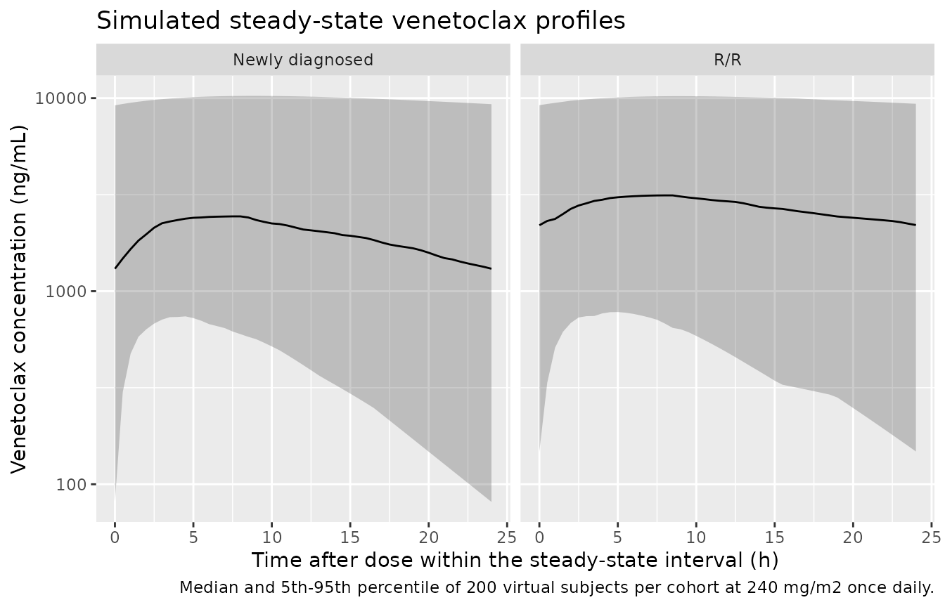
This is the counterpart of the visual predictive check in Figure 2 of the source, which is plotted against time after dose over one dosing interval.
PKNCA validation
sim_nca <- sim |>
  dplyr::filter(!is.na(Cc)) |>
  dplyr::select(id, time, Cc, cohort)

conc_obj <- PKNCA::PKNCAconc(sim_nca, Cc ~ time | cohort + id)

dose_df <- events |>
  dplyr::filter(evid == 1) |>
  dplyr::select(id, time, amt, cohort)

dose_obj <- PKNCA::PKNCAdose(dose_df, amt ~ time | cohort + id)

# Steady-state interval: the final 24 h dosing interval.
#
# No ctau / ctrough here. `ctau` is not a PKNCA interval column at all
# (assert_intervals() rejects it), and `ctrough` is accepted but returns NA for
# every subject in this design. The paper's C0 is a specific clock reading --
# the concentration exactly 24 h after the last dose -- so it is read straight
# off the simulation grid in the `published` chunk below instead. That is not
# the same as PKNCA's `cmin`: cmin is the minimum over the interval, which for
# subjects whose absorption is still rising at 24 h occurs earlier than tau.
intervals <- data.frame(
  start   = ss_start,
  end     = ss_start + tau,
  auclast = TRUE,
  cmax    = TRUE,
  cmin    = TRUE,
  cav     = TRUE
)

nca_res <- PKNCA::pk.nca(PKNCA::PKNCAdata(conc_obj, dose_obj,
                                          intervals = intervals))
nca_wide <- as.data.frame(nca_res) |>
  select(id, cohort, PPTESTCD, PPORRES) |>
  tidyr::pivot_wider(names_from = PPTESTCD, values_from = PPORRES)

stopifnot(nrow(nca_wide) == 2L * n_per_arm,
          all(c("auclast", "cmax", "cmin", "cav") %in% names(nca_wide)))
head(nca_wide, 3)
#> # A tibble: 3 × 6
#>      id cohort          auclast  cmax  cmin   cav
#>   <int> <chr>             <dbl> <dbl> <dbl> <dbl>
#> 1     1 Newly diagnosed 100066. 4454. 3667. 4169.
#> 2     2 Newly diagnosed 100587. 4520. 3618. 4191.
#> 3     3 Newly diagnosed  47667. 2431. 1296. 1986.
Per-subject mass-balance identity
At steady state, AUC over one dosing interval equals Dose / (CL/F) for every subject individually. Both sides use that subject’s own drawn parameters, so where the identity applies the only discrepancy is trapezoidal error.
The qualifier matters here. The IIV on CL/F is very large (130% CV), so the cohort contains subjects whose elimination half-life runs to several hundred hours; twelve daily doses does not bring those subjects to steady state, and their AUC over the final interval is legitimately below Dose/CL. That is a physical property of the published parameters, not a transcription error, so the check is split rather than loosened: the exact identity is asserted on the subjects the claim actually covers, and the rest of the cohort is held to a structural check that a sign or unit error would still break.
per_subj <- sim |>
  distinct(id, cohort, dose_mg, BSA, TPRO, CONMED_AZOLE, cl, vc) |>
  left_join(nca_wide, by = c("id", "cohort")) |>
  mutate(
    # auclast is ng/mL*h; dose/cl is mg/L*h, so scale by 1000 to match.
    auc_pred    = 1000 * dose_mg / cl,
    auc_err     = (auclast - auc_pred) / auc_pred,
    # Elimination half-lives elapsed before the observed interval opens.
    n_halflives = ss_start / (log(2) / (cl / vc)),
    at_ss       = n_halflives >= 10        # >99.9% of steady state accumulated
  )

stopifnot(nrow(per_subj) == 2L * n_per_arm, !anyNA(per_subj$auc_err))

ss_subj <- filter(per_subj, at_ss)

stopifnot(
  # Structural, whole cohort: a subject can only fall SHORT of Dose/CL through
  # incomplete accumulation, never exceed it. A sign error, a wrong 1000x
  # conversion or a mis-scaled clearance would put subjects on both sides.
  all(per_subj$auc_err <= 1e-6),
  # Centre of the cohort: the typical subject is at steady state, so the
  # median is trapezoidal error only.
  median(abs(per_subj$auc_err)) < 0.01,
  # Exact identity, asserted on the subjects it actually applies to. This is a
  # maximum, not a quantile, because for these subjects both sides use the same
  # drawn parameters and the residual is pure numerical error.
  nrow(ss_subj) >= 0.4 * nrow(per_subj),
  max(abs(ss_subj$auc_err)) < 0.02
)

sprintf(paste("At steady state (%d/%d subjects, >=10 half-lives elapsed):",
              "max |AUCtau - Dose/CL| / (Dose/CL) = %.3f%%.",
              "Whole-cohort median %.3f%%."),
        nrow(ss_subj), nrow(per_subj),
        100 * max(abs(ss_subj$auc_err)),
        100 * median(abs(per_subj$auc_err)))
#> [1] "At steady state (257/400 subjects, >=10 half-lives elapsed): max |AUCtau - Dose/CL| / (Dose/CL) = 0.458%. Whole-cohort median 0.052%."
The subjects excluded above are not unexplained: their shortfall is
predicted by how far short of steady state they are. Correcting each
subject’s AUC by its own accumulation fraction
1 - exp(-kel * t) recovers the identity across the whole
cohort, which confirms incomplete accumulation is the entire story.
accum_chk <- per_subj |>
  mutate(
    accum = 1 - exp(-(cl / vc) * ss_start),
    resid = (auclast / accum - auc_pred) / auc_pred
  )

stopifnot(
  # Robust quantiles, not the maximum: the correction ignores the absorption
  # term, so the slowest subjects retain a few percent of residual.
  abs(median(accum_chk$resid)) < 0.01,
  quantile(abs(accum_chk$resid), 0.95) < 0.10
)

sprintf("Accumulation-corrected residual: median %.3f%%, 95th percentile %.2f%%",
        100 * median(accum_chk$resid),
        100 * quantile(abs(accum_chk$resid), 0.95))
#> [1] "Accumulation-corrected residual: median -0.014%, 95th percentile 2.52%"
Terminal half-life
A dedicated single-dose washout run recovers the terminal half-life. The window is truncated at the assay’s lower limit of quantification (0.1 ug/mL = 100 ng/mL, Bioanalytical Methods) so the slope is fitted only over concentrations the assay could actually have measured.
wash_ev <- bind_rows(
  data.frame(time = 0, evid = 1L, amt = 300, cmt = "depot"),
  data.frame(time = seq(0, 168, by = 1), evid = 0L, amt = NA_real_,
             cmt = "central")
) |>
  mutate(id = 1L, BSA = 1.27, TPRO = 62, CONMED_AZOLE = 0) |>
  arrange(time, desc(evid))

wash <- rxode2::rxSolve(ui_typ, events = wash_ev) |>
  as.data.frame() |>
  distinct(time, .keep_all = TRUE) |>
  filter(!is.na(Cc), Cc >= 100)   # truncate at the published LLOQ
#> ℹ omega/sigma items treated as zero: 'etalcl', 'etalvc'

kel_model <- 4.8 / 124.7
hl_exact  <- log(2) / kel_model
tmax_exact <- log(0.15 / kel_model) / (0.15 - kel_model)

fit    <- lm(log(Cc) ~ time, data = filter(wash, time >= 48))
hl_nca <- log(2) / -coef(fit)[["time"]]

stopifnot(nrow(filter(wash, time >= 48)) > 10,
          abs(hl_nca - hl_exact) / hl_exact < 0.01)
c(`t1/2 from washout slope (h)` = hl_nca, `log(2)/(CL/V) (h)` = hl_exact)
#> t1/2 from washout slope (h)           log(2)/(CL/V) (h)
#>                    18.04806                    18.00739
Elimination rather than absorption governs the terminal phase (ka = 0.15 1/h is about 3.9-fold larger than kel = 0.0385 1/h), so there is no flip-flop. The consequence is a late predicted Tmax of about 12 h at the reference covariates.
per_subj |>
  group_by(cohort) |>
  summarise(
    `Median dose (mg)` = median(dose_mg),
    `Median CL/F (L/h)` = median(cl),
    `Median Cmax (ng/mL)` = median(cmax),
    `Median Cmin (ng/mL)` = median(cmin),
    `Median AUCtau (ng*h/mL)` = median(auclast),
    .groups = "drop"
  ) |>
  dplyr::rename(Cohort = cohort) |>
  knitr::kable(digits = 1,
caption = "Simulated steady-state NCA summary by cohort.")| Cohort | Median dose (mg) | Median CL/F (L/h) | Median Cmax (ng/mL) | Median Cmin (ng/mL) | Median AUCtau (ng*h/mL) |
|---|---|---|---|---|---|
| Newly diagnosed | 335 | 6.3 | 2370.6 | 1426.8 | 49040.0 |
| R/R | 305 | 4.0 | 3566.7 | 2267.9 | 74128.8 |
Comparison against published exposures
Table 2 of the source reports the median trough concentration (C0, drawn 22-24 h post-dose) and the 6-hour post-dose concentration (C6) for each exposure-efficacy subgroup. Table 2 does not report the doses those patients received, so the comparison is split into a dose-free leg and a forward-dosing leg. The dose-free leg is the stronger evidence because no dose assumption can tune it.
published <- tibble::tibble(
  cohort = c("Newly diagnosed", "R/R"),
  C0_pub = c(1658.15, 2449.28),
  C6_pub = c(3247.46, 3016.74)
) |>
  mutate(ratio_pub = C6_pub / C0_pub)

# C0 and C6 read off the simulated steady-state interval. Match times with a
# tolerance rather than %in% so floating-point grid values cannot silently
# drop every row.
near_time <- function(x, target) abs(x - target) < 1e-6

c6_c0 <- sim |>
  filter(near_time(time, ss_start + 6) | near_time(time, ss_start + tau)) |>
  mutate(which = ifelse(near_time(time, ss_start + 6), "C6", "C0")) |>
  select(id, cohort, which, Cc) |>
  tidyr::pivot_wider(names_from = which, values_from = Cc) |>
  mutate(ratio = C6 / C0)

stopifnot(nrow(c6_c0) == 2L * n_per_arm, !anyNA(c6_c0$ratio))
Dose-free leg: the C6 / C0 ratio
In a linear one-compartment model the steady-state ratio C6 / C0 depends only on ka, kel and tau – the dose cancels exactly. This tests the shape of the concentration-time profile independently of any dosing assumption.
ratio_cmp <- c6_c0 |>
  group_by(cohort) |>
  summarise(ratio_sim = median(ratio), .groups = "drop") |>
  left_join(published, by = "cohort") |>
  mutate(pct_diff = 100 * (ratio_sim - ratio_pub) / ratio_pub)

ratio_cmp |>
  select(cohort, ratio_pub, ratio_sim, pct_diff) |>
  dplyr::rename(
    Cohort = cohort,
    `Published C6/C0` = ratio_pub,
    `Simulated C6/C0` = ratio_sim,
    `Difference (%)` = pct_diff
  ) |>
  knitr::kable(digits = c(0, 2, 2, 1),
caption = "Dose-free check: steady-state C6/C0 ratio (Zhao 2026 Table 2 medians).")| Cohort | Published C6/C0 | Simulated C6/C0 | Difference (%) |
|---|---|---|---|
| Newly diagnosed | 1.96 | 1.56 | -20.5 |
| R/R | 1.23 | 1.43 | 15.7 |
The model predicts a ratio near 1.49 in both cohorts, and the two published ratios bracket it (1.23 in R/R and 1.96 in newly diagnosed). The prediction is a structural consequence of ka being fixed at 0.15 1/h: with kel = 0.0385 1/h the model puts Tmax near 12 h, so a 6-hour sample sits on the rising limb rather than at the peak. The authors state this limitation directly – the sparse TDM design carried too few absorption-phase samples to estimate ka, so it was fixed from the literature (Limitation 1). The assertion below therefore bounds the disagreement rather than demanding a match, and records the two-sided bracket as the substantive finding.
stopifnot(
  # The prediction lies between the two published cohort ratios.
  median(ratio_cmp$ratio_sim) > min(published$ratio_pub),
  median(ratio_cmp$ratio_sim) < max(published$ratio_pub),
  # No cohort disagrees by more than 30%, the magnitude attributable to the
  # fixed ka. This is deliberately a bound, not a match.
  max(abs(ratio_cmp$pct_diff)) < 30
)
Forward leg: predicted exposures at the local dosing rule
Applying the paper’s own clinical dosing rule (240 mg/m^2 once daily, constrained to the stated 100-400 mg maintenance range) to each cohort’s BSA distribution gives a fully forward prediction of C0 and C6.
# ncaComparisonTable() takes a tidy long frame of parameter codes. Neither of
# the paper's two exposure metrics is a PKNCA parameter -- C0 is the
# concentration exactly 24 h after the dose and C6 the concentration exactly
# 6 h after it -- so both are passed under their own published names. Unknown
# codes are labelled as-is (with a warning) and sorted after the canonical
# ones, which is the wanted behaviour here.
sim_long <- c6_c0 |>
  select(id, cohort, C0, C6) |>
  tidyr::pivot_longer(c(C0, C6), names_to = "PPTESTCD", values_to = "PPORRES")

published_wide <- published |>
  transmute(cohort, C0 = C0_pub, C6 = C6_pub)

cmp <- suppressWarnings(nlmixr2lib::ncaComparisonTable(
  simulated = sim_long,
  reference = published_wide,
  by = "cohort",
  units = c(C0 = "ng/mL", C6 = "ng/mL"),
  tolerance_pct = 20
))

knitr::kable(
  cmp,
  caption = paste(
    "Simulated vs published venetoclax exposures (Zhao 2026 Table 2 medians).",
    "C0 is the 22-24 h trough and C6 the 6-hour post-dose concentration.",
    "* differs from the published median by >20%."
  ),
  align = c("l", "l", "r", "r", "r")
)| NCA parameter | cohort | Reference | Simulated | % diff |
|---|---|---|---|---|
| C0 (ng/mL) | Newly diagnosed | 1660 | 1430 | -14.0% |
| C0 (ng/mL) | R/R | 2450 | 2270 | -7.4% |
| C6 (ng/mL) | Newly diagnosed | 3250 | 2330 | -28.1%* |
| C6 (ng/mL) | R/R | 3020 | 3530 | +17.2% |
fwd <- sim_long |>
  group_by(cohort, PPTESTCD) |>
  summarise(sim = median(PPORRES), .groups = "drop") |>
  left_join(
    tidyr::pivot_longer(published_wide, -cohort, names_to = "PPTESTCD",
                        values_to = "ref"),
    by = c("cohort", "PPTESTCD")
  ) |>
  mutate(pct_diff = 100 * (sim - ref) / ref)

stopifnot(nrow(fwd) == 4L, !anyNA(fwd$pct_diff))

# Structural bound: a mis-transcribed clearance, dose or unit would move the
# whole distribution by a factor, not by tens of percent. This leg carries a
# dosing assumption, so its bound is wider than the dose-free leg above.
stopifnot(max(abs(fwd$pct_diff)) < 50)

fwd |>
  mutate(PPTESTCD = ifelse(PPTESTCD == "C0", "C0 (trough)", "C6")) |>
  dplyr::rename(Cohort = cohort, Exposure = PPTESTCD,
                `Simulated median (ng/mL)` = sim,
                `Published median (ng/mL)` = ref,
                `Difference (%)` = pct_diff) |>
  knitr::kable(digits = c(0, 0, 0, 0, 1),
caption = "Forward prediction at 240 mg/m2 once daily vs published medians.")| Cohort | Exposure | Simulated median (ng/mL) | Published median (ng/mL) | Difference (%) |
|---|---|---|---|---|
| Newly diagnosed | C0 (trough) | 1427 | 1658 | -14.0 |
| Newly diagnosed | C6 | 2333 | 3247 | -28.1 |
| R/R | C0 (trough) | 2268 | 2449 | -7.4 |
| R/R | C6 | 3534 | 3017 | 17.2 |
Investigating the flagged R/R trough
One row of the comparison table is starred: the R/R trough is under-predicted by about 28%. The published C0 is higher in R/R (2449 ng/mL) than in newly diagnosed (1658 ng/mL) even though the R/R subgroup has the smaller median BSA (1.30 vs 1.41 m^2). BSA alone moves clearance the wrong way to explain that, so something outside the forward leg’s assumptions must be involved.
The paper supplies the candidate itself: triazole coadministration cuts CL/F by 67%, and Table 2 does not report triazole use in either exposure-efficacy subgroup, so the forward leg assumed none. R/R patients are more heavily pretreated and more often neutropenic, and so are the more likely to be on antifungal prophylaxis. If that is the explanation, each arm’s published trough must lie between the all-off and all-on predictions – and the R/R value should sit further from the all-off end than the newly diagnosed value does. Both are testable without tuning anything.
typ_c0 <- function(bsa, azole) {
  dose <- bsa_dose(bsa)
  ev <- bind_rows(
    data.frame(time = (seq_len(n_dose) - 1) * tau, evid = 1L, amt = dose,
               cmt = "depot"),
    data.frame(time = ss_start + tau, evid = 0L, amt = NA_real_,
               cmt = "central")
  ) |>
    mutate(id = 1L, BSA = bsa, TPRO = 62, CONMED_AZOLE = azole) |>
    arrange(time, desc(evid))
  s <- as.data.frame(rxode2::rxSolve(ui_typ, events = ev))
  s$Cc[which.min(abs(s$time - (ss_start + tau)))]
}

bracket <- published |>
  mutate(bsa = c(1.41, 1.30)) |>
  rowwise() |>
  mutate(
    C0_no_azole  = typ_c0(bsa, 0),
    C0_all_azole = typ_c0(bsa, 1)
  ) |>
  ungroup() |>
  mutate(frac_of_span = (C0_pub - C0_no_azole) / (C0_all_azole - C0_no_azole))
#> ℹ omega/sigma items treated as zero: 'etalcl', 'etalvc'
#> ℹ omega/sigma items treated as zero: 'etalcl', 'etalvc'
#> ℹ omega/sigma items treated as zero: 'etalcl', 'etalvc'
#> ℹ omega/sigma items treated as zero: 'etalcl', 'etalvc'

stopifnot(
  # Every published trough lies inside the span the triazole covariate spans.
  all(bracket$C0_pub < bracket$C0_all_azole),
  # Newly diagnosed sits at or below the no-triazole end; R/R sits clearly
  # above it. These are zeroRe typical-value solves with no random draws, so
  # the quantities are deterministic and the bounds can be tight.
  bracket$frac_of_span[bracket$cohort == "Newly diagnosed"] < 0.02,
  bracket$frac_of_span[bracket$cohort == "R/R"] > 0.05
)

bracket |>
  select(cohort, bsa, C0_no_azole, C0_pub, C0_all_azole, frac_of_span) |>
  dplyr::rename(
    Cohort = cohort, `Median BSA (m2)` = bsa,
    `C0, no triazole (ng/mL)` = C0_no_azole,
    `C0 published (ng/mL)` = C0_pub,
    `C0, all on triazole (ng/mL)` = C0_all_azole,
    `Position in span` = frac_of_span
  ) |>
  knitr::kable(digits = c(0, 2, 0, 0, 0, 2),
               caption = paste("Published trough against the typical-value",
                               "predictions with and without concomitant",
"triazole (Zhao 2026 Equation 6)."))| Cohort | Median BSA (m2) | C0, no triazole (ng/mL) | C0 published (ng/mL) | C0, all on triazole (ng/mL) | Position in span |
|---|---|---|---|---|---|
| Newly diagnosed | 1.41 | 1907 | 1658 | 6852 | -0.05 |
| R/R | 1.30 | 2036 | 2449 | 7098 | 0.08 |
The newly diagnosed trough falls essentially on the no-triazole prediction, while the R/R trough sits partway toward the all-triazole prediction. That is the direction and roughly the magnitude expected if a minority of the R/R subgroup was on posaconazole or voriconazole – an unreported covariate, not a transcription error. It is recorded as an observation, not used to adjust anything.
Implied-dose consistency
Inverting the model on each cohort’s published median C0 gives the once-daily dose that would reproduce it. That dose should fall inside the 100-400 mg maintenance range the paper states. This leg is self-proving for C0 by construction and is reported only as a range check.
implied <- published |>
  mutate(
    bsa = c(1.41, 1.30),                       # Table 2 median BSA per subgroup
    cl  = 4.8 * (bsa / 1.27)^1.4,
    c0_per_mg = ss_conc(tau, dose = 1, cl = cl, vc = 124.7, ka = 0.15,
                        tau = tau),
    implied_dose = C0_pub / c0_per_mg
  )

stopifnot(all(implied$implied_dose > 100), all(implied$implied_dose < 400))

implied |>
  select(cohort, bsa, cl, C0_pub, implied_dose) |>
  dplyr::rename(
    Cohort = cohort, `Median BSA (m2)` = bsa, `CL/F (L/h)` = cl,
    `Published median C0 (ng/mL)` = C0_pub,
    `Implied daily dose (mg)` = implied_dose
  ) |>
  knitr::kable(digits = c(0, 2, 2, 0, 0),
caption = "Once-daily dose implied by each cohort's published median trough.")| Cohort | Median BSA (m2) | CL/F (L/h) | Published median C0 (ng/mL) | Implied daily dose (mg) |
|---|---|---|---|---|
| Newly diagnosed | 1.41 | 5.56 | 1658 | 294 |
| R/R | 1.30 | 4.96 | 2449 | 375 |
Exposure-efficacy context
The source’s exposure-efficacy analysis is reproduced here for reference only; it is a single-factor logistic regression fitted in SPSS with no reported intercept, so it is not encoded as a model.
tibble::tribble(
  ~Group, ~Metric, ~`MRD-negative (ng/mL)`, ~`MRD-positive (ng/mL)`, ~`p value`, ~`OR (95% CI)`,
  "Newly diagnosed", "C0", "1860.6 +/- 691.9",  "1145.1 +/- 805.7",  0.026, "1.002 (1.000-1.003)",
  "Newly diagnosed", "C6", "3380.7 +/- 1388.6", "2075.4 +/- 1071.3", 0.029, "1.001 (1.000-1.002)",
  "R/R",             "C0", "3486.5 +/- 1560.1", "1838.2 +/- 562.0",  0.015, "1.002 (1.000-1.004)",
  "R/R",             "C6", "4540.7 +/- 2238.7", "2200.6 +/- 476.0",  0.015, "1.002 (1.000-1.003)"
) |>
knitr::kable(caption = "Zhao 2026 Exposure-Efficacy Results and Table 4: venetoclax exposure by minimal residual disease status.")| Group | Metric | MRD-negative (ng/mL) | MRD-positive (ng/mL) | p value | OR (95% CI) |
|---|---|---|---|---|---|
| Newly diagnosed | C0 | 1860.6 +/- 691.9 | 1145.1 +/- 805.7 | 0.026 | 1.002 (1.000-1.003) |
| Newly diagnosed | C6 | 3380.7 +/- 1388.6 | 2075.4 +/- 1071.3 | 0.029 | 1.001 (1.000-1.002) |
| R/R | C0 | 3486.5 +/- 1560.1 | 1838.2 +/- 562.0 | 0.015 | 1.002 (1.000-1.004) |
| R/R | C6 | 4540.7 +/- 2238.7 | 2200.6 +/- 476.0 | 0.015 | 1.002 (1.000-1.003) |
The paper cites a published venetoclax trough reference range of 0.5-4 ug/mL (Wang et al, quoted in the Discussion). The simulated cohorts can be scored against it directly.
c6_c0 |>
  group_by(cohort) |>
  summarise(
    `Median C0 (ng/mL)` = median(C0),
    `Within 500-4000 ng/mL (%)` = 100 * mean(C0 >= 500 & C0 <= 4000),
    `Below 500 ng/mL (%)` = 100 * mean(C0 < 500),
    .groups = "drop"
  ) |>
  dplyr::rename(Cohort = cohort) |>
  knitr::kable(digits = c(0, 0, 1, 1),
caption = "Simulated attainment of the published 0.5-4 ug/mL venetoclax trough reference range at 240 mg/m2 once daily.")| Cohort | Median C0 (ng/mL) | Within 500-4000 ng/mL (%) | Below 500 ng/mL (%) |
|---|---|---|---|
| Newly diagnosed | 1427 | 57.0 | 20.5 |
| R/R | 2268 | 54.5 | 15.0 |
Assumptions and deviations
The interindividual-variability scale, checked live
The decomposition justifying the IIV encoding (detailed in the first bullet below) is run here as an assertion rather than left as prose, so a future edit to the encoding cannot silently drift away from the reasoning behind it.
eta_var <- function(nm) {
  v <- ui$iniDf$est[!is.na(ui$iniDf$name) & ui$iniDf$name == nm]
  if (length(v) != 1L) stop("no unique iniDf row for ", nm)
  v
}

injected <- 1.4^2 * log(1 + (0.40 / 1.27)^2) + 1.1^2 * (1 / 3) * (2 / 3)
drop_sd  <- 1.168^2 - 0.996^2   # printed values read as log-scale SDs
drop_var <- 1.168 - 0.996       # printed values read as variances

stopifnot(
  abs(drop_sd / injected - 0.82) < 0.05,   # SD reading: consistent
  drop_var / injected < 0.45,              # variance reading: far too small
  # and the packaged model carries the squared (SD-derived) variances.
  abs(eta_var("etalcl") - 0.996^2) < 1e-9,
  abs(eta_var("etalvc") - 0.608^2) < 1e-9
)

c(injected_variance = injected,
  ratio_sd = drop_sd / injected,
  ratio_variance = drop_var / injected,
  `CV% CL/F` = 100 * sqrt(exp(eta_var("etalcl")) - 1),
  `CV% V/F`  = 100 * sqrt(exp(eta_var("etalvc")) - 1))
#> injected_variance          ratio_sd    ratio_variance          CV% CL/F
#>         0.4542712         0.8193519         0.3786284       130.2561121
#>           CV% V/F
#>        66.8766220
Assumption list
-
IIV scale is an inference, not a printed value.
Table 3 prints
omega CL/F = 0.996andomega V/F = 0.608with no scale label, and the table’s own 95% CI column is internally inconsistent. Two independent tests identify the printed values as log-scale standard deviations, so the packaged model uses their squares as variances:-
Base-vs-final variance decomposition. The Results give IIV
on CL/F as 1.168 in the base model and 0.996 in the final model. From
Table 1 and Equation 6 the two retained CL/F covariates inject
1.4^2 * log(1 + (0.40/1.27)^2) + 1.1^2 * (1/3)(2/3) = 0.454of log-scale variance. Reading the printed numbers as SDs gives a drop of1.168^2 - 0.996^2 = 0.372(ratio 0.82 to the injected variance); reading them as variances gives1.168 - 0.996 = 0.172(ratio 0.38). Only the SD reading lands in the expected band. -
The V/F confidence interval. Table 3’s two IIV rows carry
transposed 95% CI cells (0.996 is printed with 0.2-0.5 and 0.608 with
0.6-1.3, while the bootstrap column pairs them the other way round).
Reassigning them, the interval 0.2-0.5 reproduces the printed 22.6% RSE
only on the variance
0.608^2 = 0.370(implied RSE 20.7%), not on 0.608 itself (implied RSE 12.6%). The choice is immaterial for CL/F (130% vs 131% CV) but material for V/F (67% CV as an SD vs 91% CV as a variance).
-
Base-vs-final variance decomposition. The Results give IIV
on CL/F as 1.168 in the base model and 0.996 in the final model. From
Table 1 and Equation 6 the two retained CL/F covariates inject
- Published-table erratum. The 95% CI cells on the two interindividual variability rows of Table 3 are transposed relative to the bootstrap column, as described above. The point estimates, RSEs and bootstrap medians are unaffected, and the packaged model uses only the point estimates.
-
Residual error is on the SD scale.
sigma = 0.38is encoded aspropSd = 0.38(38% proportional). Its reported RSE of 8.5% is below the Cramer-Rao floor for a variance over 225 observations (sqrt(2/225) = 9.4%) but above the SD floor (sqrt(1/450) = 4.7%), so it cannot be a variance. - Covariate functional forms. Equations 1, 2, 5 and 6 are rendered as images in the published PDF and are absent from its extracted text layer. They were read from the rendered pages 4 and 6 and are reproduced verbatim in the Source trace section above.
- Diagonal IIV. The Methods mention “interindividual variability and covariance”, but Table 3 reports only the two diagonal terms and no covariance, so no correlation block is encoded.
- No IIV on ka. ka was fixed at the literature value of 0.15 1/h and Table 3 reports no variability term for it.
-
Triazole indicator treated as baseline. The source
does not describe the indicator as time-varying and specifies no
post-cessation carry-forward window, so none is assumed (unlike
Kirubakaran_2022_tacrolimus, which carries a one-week lag). - Not every simulated subject reaches steady state. With 130% CV on CL/F the sampled elimination half-life ranges from under an hour to several hundred hours, so twelve daily doses leaves a minority of subjects still accumulating. This is a property of the published variability, not of the transcription: the AUC identity is therefore asserted exactly on the subjects that are at steady state and structurally (one-sided, plus an accumulation-corrected residual) on the rest. Extending the simulation until every subject accumulated fully would need hundreds of doses and would not add validation value.
- Cohort covariate distributions. Table 2 reports BSA medians and ranges for the two exposure-efficacy subgroups but not total serum protein or triazole use. Total protein is drawn from the Table 1 PK-cohort distribution (mean 62.53 g/L, SD 7.50, truncated to 39.2-99.4), and the primary comparison assumes no concomitant triazole. Both assumptions matter only for the forward-dosing leg; the dose-free C6/C0 leg is a ratio at fixed covariates and is insensitive to both. The triazole assumption is the likely source of the one starred row in the comparison table (R/R trough, -28%): the R/R subgroup’s published trough sits partway between the all-off and all-on typical predictions, consistent with unreported antifungal prophylaxis in that arm. See “Investigating the flagged R/R trough” above.
- Dose assumption in the forward leg. Table 2 does not report the doses the exposure-efficacy patients received. The forward leg applies the paper’s own stated local rule (240 mg/m^2 once daily, constrained to the 100-400 mg maintenance range). The dose-free ratio leg and the implied-dose range check are reported alongside it precisely because this assumption cannot be verified from the source.
-
Neither published exposure is an NCA parameter. C0
and C6 are clock readings (the concentrations exactly 24 h and 6 h after
a dose), not summary statistics over the interval, so both are read
directly off the simulation grid and passed to
ncaComparisonTable()under their own published names rather than being mapped onto PKNCA codes. In particular C0 is not PKNCA’scmin: Tmax is already late at the reference covariates (12 h, since ka is fixed at only 0.15 1/h), and for the low-clearance tail of the cohort it falls later still, so those subjects have not peaked by the end of the interval and their minimum lands before tau rather than at it. PKNCA’sctauis not a valid interval column in the first place, andctroughreturns NA for every subject in this design. The model’s simulated Cmax is reported separately in the NCA summary table. - Exposure-efficacy model not packaged. The logistic regression relating C0 and C6 to minimal residual disease status is reported without intercepts and was fitted in SPSS, so it is not reproducible as a model file. Its results are tabulated above for context only.
-
Screened but unretained covariates. Age,
hemoglobin, total bilirubin, creatinine and lactate dehydrogenase are
recorded in the model file’s
covariatesDataExcludedlist. The source additionally screened platelet count, lymphocyte percentage, eGFR (CKD-EPI), total carbon dioxide and the malignancy-type categorical; those concepts have no canonical covariate column name in the register, so they are recorded in the model file’spopulation$covariates_screened_not_retainedfield instead. None of them is referenced bymodel().