Model and source
- Citation: Zhao W, Piana C, Danhof M, Burger D, Della Pasqua O, Jacqz-Aigrain E. Population pharmacokinetics of abacavir in infants, toddlers and children. Br J Clin Pharmacol. 2013;75(6):1525-1535. doi:10.1111/bcp.12024
- Description: Two-compartment population PK model for oral abacavir in HIV-infected infants, toddlers, and children (Zhao 2013); body weight is the only retained covariate (allometric on CL/F and V1/F with estimated exponents and reference weight 17.6 kg).
- Article: https://doi.org/10.1111/bcp.12024
This vignette accompanies the abacavir popPK model
from Zhao 2013 (pooled paediatric meta-analysis across three trials). A
separate nlmixr2lib entry, Archary_2019_abacavir, holds the
same drug in a different paediatric population (severely malnourished,
South African inpatients) and is appropriate for that population – both
models are abacavir popPK; choose the one closer to the population you
are simulating.
Population
Zhao 2013 reports a pooled paediatric meta-analysis of three clinical trials in HIV type-1-infected children: PENTA 13 (n = 14, 2.14-12.84 years), PENTA 15 (n = 18, 0.42-2.81 years), and the ARROW pharmacokinetic substudy (n = 37, 3.62-12.54 years). The overall cohort is 69 children spanning 0.42-12.84 years and 7.6-60.9 kg (median 5.66 years, 17.6 kg; Table 1 of the source). Children received either a weight-normalised 16 mg/kg/day regimen or WHO weight-band fixed dosing (300 / 450 / 600 mg per day) split as twice daily (8 mg/kg BID or 150-300 mg BID) or once daily; both tablet and oral solution formulations were used. Steady-state pharmacokinetic samples were collected at T0, T1, T2, T3, T4, T6, T8, and T12 h after dosing (plus T24 h for the once-daily regimen). The pooled dataset contains 1065 abacavir concentrations across 138 pharmacokinetic profiles.
The same information is available programmatically:
readModelDb("Zhao_2013_abacavir")$population after the
model is loaded.
Source trace
Per-parameter origin (also recorded as in-file comments next to each
ini() entry of
inst/modeldb/specificDrugs/Zhao_2013_abacavir.R):
| Equation / parameter | Value | Source location |
|---|---|---|
lka |
log(0.913) | Zhao 2013 Table 2 (Ka = 0.913 /h) |
lcl |
log(20.1) | Zhao 2013 Table 2 (CL/F_ref = 20.1 L/h at 17.6 kg) |
lvc |
log(13.0) | Zhao 2013 Table 2 (V1/F_ref = 13.0 L at 17.6 kg) |
lvp |
log(13.5) | Zhao 2013 Table 2 (V2/F = 13.5 L) |
lq |
log(2.0) | Zhao 2013 Table 2 (Q/F = 2.0 L/h) |
e_wt_cl |
0.802 | Zhao 2013 Table 2 (theta_1 allometric exponent on CL/F) |
e_wt_vc |
0.810 | Zhao 2013 Table 2 (theta_2 allometric exponent on V1/F) |
etalcl |
0.08763 | Zhao 2013 Table 2 (combined 21.9 % BSV + 20.4 % IOV on CL/F; see Assumptions and deviations) |
etalvc |
0.20509 | Zhao 2013 Table 2 (47.7 % CV IIV on V1/F; omega^2 = log(1 + 0.477^2)) |
etalvp |
0.28555 | Zhao 2013 Table 2 (57.5 % CV IIV on V2/F; omega^2 = log(1 + 0.575^2)) |
etalq |
0.16608 | Zhao 2013 Table 2 (42.5 % CV IIV on Q/F; omega^2 = log(1 + 0.425^2)) |
propSd |
0.382 | Zhao 2013 Table 2 (38.2 % proportional residual error) |
| Reference weight | 17.6 kg | Zhao 2013 Results (“the reference weight was the median value of our population, 17.6 kg”) |
d/dt(depot), d/dt(central),
d/dt(peripheral1)
|
n/a | Zhao 2013 Results (two-compartment model with first-order absorption and first-order elimination) |
Cc <- central / vc |
n/a | Standard apparent-clearance parameterisation; dose mg, volume L -> mg/L |
Cc ~ prop(propSd) |
n/a | Zhao 2013 Results (“Residual variability was best described by a proportional model”) |
Virtual cohort
Original observed data are not publicly available. The cohort below is a virtual reproduction of the paper’s two subpopulation simulations (infants + toddlers, and children) used to compare against the published steady-state Cmax and AUC0-12 values:
- Infants and toddlers (n = 21 in the source; age 0.42-2.81 years; WT range ~7.6-15.8 kg, median 11.6 kg – taken from PENTA 15 demographics in Table 1).
- Children (n = 48 in the source; age 3.58-12.84 years; pooled from ARROW (n = 37, mean 20.3 kg, SD 4.0, range 14-29.8 kg) and PENTA 13 (n = 14, mean 23.9 kg, SD 13.2, range 14-60.9 kg) – the PENTA 13 long right tail (up to 60.9 kg) makes the children subgroup considerably wider than ARROW alone).
Both subgroups are simulated at the standard regimen of 8 mg/kg twice daily until steady state.
set.seed(20130428L)

n_per_group  <- 100L    # subjects per subpopulation
ndoses       <- 14L     # 7 days of BID dosing -> steady state
tau          <- 12      # h, BID interval
sample_hours <- c(0, 0.25, 0.5, 0.75, 1, 1.5, 2, 3, 4, 6, 8, 10, 12)
dose_window  <- (ndoses - 1L) * tau   # 156 h: last dose time

draw_wt_mix <- function(n) {
  # Children subgroup is a mixture of ARROW (n = 37) and PENTA 13 (n = 14)
  # demographics; 37 / (37 + 14) = 72.5 % ARROW, 27.5 % PENTA 13.
  is_penta13 <- stats::runif(n) < (14 / (14 + 37))
  arrow      <- pmin(pmax(stats::rnorm(n, 20.3,  4.0), 14, 29.8))
  penta13    <- pmin(pmax(stats::rnorm(n, 23.9, 13.2), 14, 60.9))
  ifelse(is_penta13, penta13, arrow)
}

# Helper: build one cohort. WT is sampled per subject from the
# subgroup-specific weight distribution and held constant over the
# simulation. Dose is computed per subject as 8 mg/kg * WT and given
# BID for 7 days.
make_cohort <- function(n, wt_draw, cohort_label, id_offset) {
  wt <- wt_draw(n)
  ids <- id_offset + seq_len(n)
  dose_amt <- 8 * wt   # 8 mg/kg per dose

  dose_rows <- tibble::tibble(
    id   = rep(ids, each = ndoses),
    time = rep(seq(0, by = tau, length.out = ndoses), times = n),
    amt  = rep(dose_amt, each = ndoses),
    evid = 1L,
    cmt  = 1L,
    WT   = rep(wt, each = ndoses)
  )
  obs_rows <- tibble::tibble(
    id   = rep(ids, each = length(sample_hours)),
    time = rep(dose_window + sample_hours, times = n),
    amt  = 0,
    evid = 0L,
    cmt  = NA_integer_,
    WT   = rep(wt, each = length(sample_hours))
  )
  dplyr::bind_rows(dose_rows, obs_rows) |>
    dplyr::mutate(cohort = cohort_label) |>
    dplyr::arrange(id, time, dplyr::desc(evid))
}

events <- dplyr::bind_rows(
  make_cohort(
    n_per_group,
    wt_draw = function(n) pmin(pmax(stats::rnorm(n, 11.5, 2.3), 7.6, 15.8)),
    cohort_label = "Infants and toddlers",
    id_offset = 0L
  ),
  make_cohort(
    n_per_group,
    wt_draw = draw_wt_mix,
    cohort_label = "Children",
    id_offset = 1000L
  )
)

stopifnot(!anyDuplicated(unique(events[, c("id", "time", "evid")])))
Simulation
mod <- rxode2::rxode2(readModelDb("Zhao_2013_abacavir"))
#> ℹ parameter labels from comments will be replaced by 'label()'

sim <- rxode2::rxSolve(
  mod,
  events = events,
  keep   = c("WT", "cohort")
) |>
  as.data.frame()
For deterministic typical-value lines (reproducing the paper’s geometric-mean profile without IIV / residual scatter):
mod_typical <- mod |> rxode2::zeroRe()
sim_typical <- rxode2::rxSolve(
mod_typical,
events = events,
keep = c("WT", "cohort")
) |>
as.data.frame()
#> ℹ omega/sigma items treated as zero: 'etalcl', 'etalvc', 'etalvp', 'etalq'
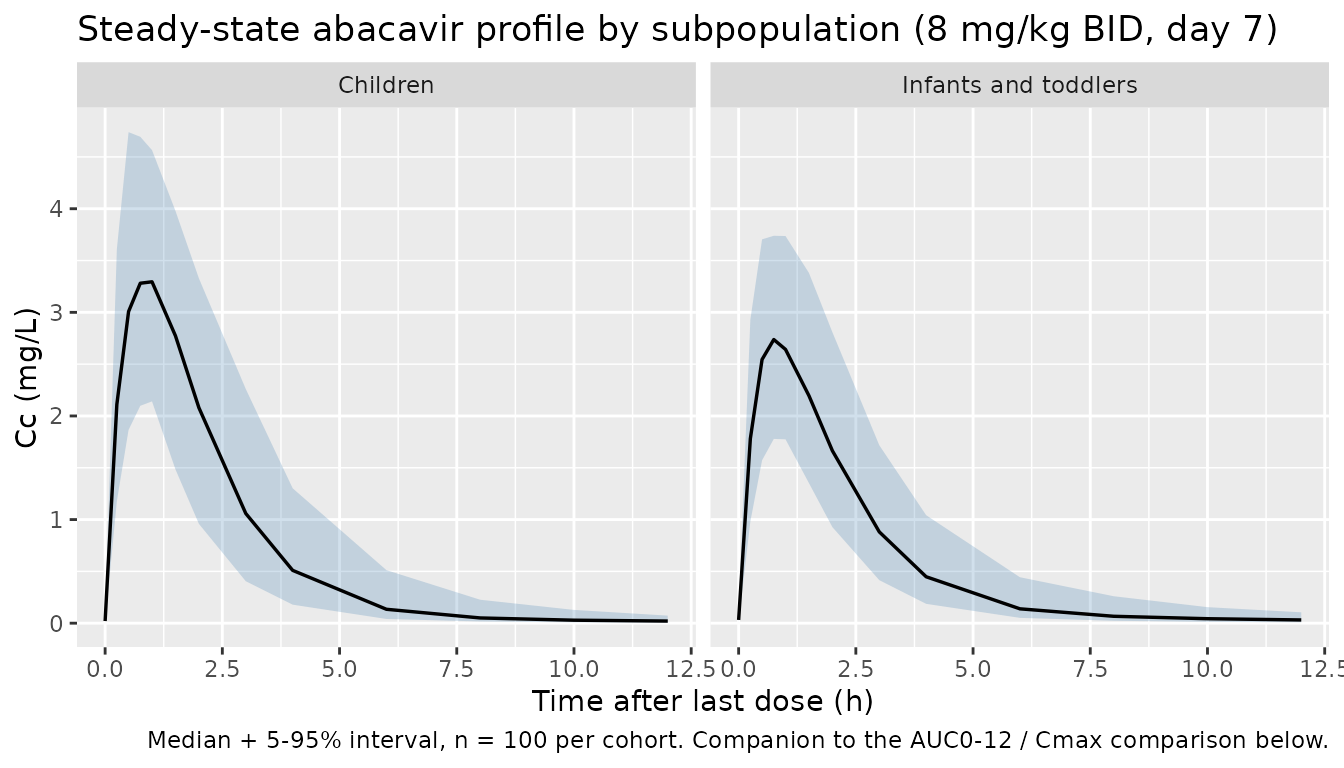
#> Warning: multi-subject simulation without without 'omega'Steady-state concentration-time profile by subpopulation
The plot below shows the simulated last-dose-interval VPC (median + 5-95 percentile band) for both subpopulations at the standard 8 mg/kg BID regimen.
sim_ss <- sim |>
  dplyr::filter(time >= dose_window, !is.na(Cc)) |>
  dplyr::mutate(tau_time = time - dose_window)

sim_quantiles <- sim_ss |>
  dplyr::group_by(cohort, tau_time) |>
  dplyr::summarise(
    Q05 = stats::quantile(Cc, 0.05, na.rm = TRUE),
    Q50 = stats::quantile(Cc, 0.50, na.rm = TRUE),
    Q95 = stats::quantile(Cc, 0.95, na.rm = TRUE),
    .groups = "drop"
  )

ggplot(sim_quantiles, aes(tau_time, Q50)) +
  geom_ribbon(aes(ymin = Q05, ymax = Q95), alpha = 0.25, fill = "steelblue") +
  geom_line(linewidth = 0.6) +
  facet_wrap(~ cohort) +
  labs(
    x = "Time after last dose (h)",
    y = "Cc (mg/L)",
    title = "Steady-state abacavir profile by subpopulation (8 mg/kg BID, day 7)",
    caption = "Median + 5-95% interval, n = 100 per cohort. Companion to the AUC0-12 / Cmax comparison below."
  )
PKNCA validation
NCA on the last dosing interval (steady-state) for each subpopulation:
pkn_in <- sim |>
  dplyr::filter(time >= dose_window, !is.na(Cc)) |>
  dplyr::mutate(tau_time = time - dose_window,
                treatment = cohort) |>
  dplyr::select(id, time = tau_time, Cc, treatment)

# Defensive guarantee: time = 0 row per (id, treatment); pre-dose at
# steady state the concentration is Ctrough, not 0, but we already have
# tau_time = 0 in sample_hours so the row is present. The bind-rows
# pattern below is a no-op safety net (distinct collapses duplicates).
pkn_in <- dplyr::bind_rows(
  pkn_in,
  pkn_in |> dplyr::distinct(id, treatment) |>
    dplyr::mutate(time = 0,
                  Cc = pkn_in |>
                    dplyr::filter(time == 0) |>
                    dplyr::pull(Cc) |>
                    stats::median(na.rm = TRUE))
) |>
  dplyr::distinct(id, treatment, time, .keep_all = TRUE) |>
  dplyr::arrange(id, treatment, time)

# One dose per subject at tau_time = 0 representing the steady-state dose.
dose_pkn <- events |>
  dplyr::filter(evid == 1L, time == dose_window) |>
  dplyr::mutate(treatment = cohort, time = 0) |>
  dplyr::select(id, time, amt, treatment)

conc_obj <- PKNCA::PKNCAconc(pkn_in, Cc ~ time | treatment + id)
dose_obj <- PKNCA::PKNCAdose(dose_pkn, amt ~ time | treatment + id,
                             route = "extravascular")

intervals <- data.frame(
  start   = 0,
  end     = 12,
  cmax    = TRUE,
  tmax    = TRUE,
  auclast = TRUE
)

nca_data <- PKNCA::PKNCAdata(conc_obj, dose_obj, intervals = intervals)
nca_res  <- PKNCA::pk.nca(nca_data)
Comparison against published values
Zhao 2013 reports the model-predicted steady-state geometric-mean Cmax and AUC0-12 for the standard 8 mg/kg BID regimen for each subpopulation:
- Infants and toddlers: Cmax = 2.5 mg/L, AUC0-12 = 6.1 mg*h/L
- Children: Cmax = 3.6 mg/L, AUC0-12 = 8.7 mg*h/L
The simulated values are summarised as the geometric mean across the virtual cohort (n = 100 per subpopulation) to match the paper’s geometric-mean summary statistic.
# Compute geometric mean of simulated Cmax / AUClast per cohort, in the
# same row shape ncaComparisonTable() expects (treatment + PPTESTCD +
# PPORRES; one row per subject-parameter pair).
sim_long <- as.data.frame(nca_res$result) |>
  dplyr::filter(PPTESTCD %in% c("cmax", "auclast")) |>
  dplyr::group_by(treatment, PPTESTCD) |>
  dplyr::summarise(
    PPORRES = exp(mean(log(PPORRES), na.rm = TRUE)),
    .groups = "drop"
  )

reference <- tibble::tribble(
  ~treatment,             ~cmax, ~auclast,
  "Infants and toddlers",  2.5,   6.1,
  "Children",              3.6,   8.7
)

cmp <- nlmixr2lib::ncaComparisonTable(
  simulated     = sim_long,
  reference     = reference,
  by            = "treatment",
  units         = c(cmax = "mg/L", auclast = "mg*h/L"),
  tolerance_pct = 20
)
knitr::kable(
  cmp,
  caption = paste(
    "Simulated steady-state geometric-mean Cmax and AUC0-12",
    "(8 mg/kg BID, n = 100 per cohort) vs published values in",
    "Zhao 2013 Results section. * differs from reference by >20%."
  )
)| NCA parameter | treatment | Reference | Simulated | % diff |
|---|---|---|---|---|
| Cmax (mg/L) | Infants and toddlers | 2.5 | 2.77 | +11.0% |
| Cmax (mg/L) | Children | 3.6 | 3.39 | -5.9% |
| AUClast (mg*h/L) | Infants and toddlers | 6.1 | 7.12 | +16.8% |
| AUClast (mg*h/L) | Children | 8.7 | 8.41 | -3.4% |
Assumptions and deviations
-
BSV + IOV on CL/F collapsed onto a single etalcl.
Zhao 2013 Table 2 reports two separate variance components on apparent
clearance: between-subject variability (21.9 % CV) and inter-occasion
variability (20.4 % CV), coupled additively in NONMEM
(
CL_ij = TVCL * exp(eta_i + kappa_ij)). nlmixr2’s library models typically simulate a single-occasion forward profile, so the two log-scale variances are added (omega^2 = 0.04686 + 0.04077 = 0.08763) and applied throughetalcl. This matches the Birgersson 2016 artemisinin convention. Consumers who need the verbatim BSV-only profile can overrideetalclto log(1 + 0.219^2) = 0.04686. -
AGE, gender, and formulation tested but not
retained. Zhao 2013 Results section reports that age, body
weight, and formulation each produced a significant OFV drop in forward
selection on CL/F, but only the effect of body weight on CL/F and V1/F
survived backward elimination. These three covariates are recorded under
covariatesDataExcludedin the model file so the provenance of the paper’s covariate screen is preserved without producing convention warnings. -
Allometric exponents estimated, not fixed at 0.75 /
1. Zhao 2013 estimated both allometric exponents from the
paediatric cohort (0.802 for CL/F, RSE 11.6 %; 0.810 for V1/F, RSE 23.3
%). The model file uses the estimated point estimates without wrapping
them in
fixed(), matching the paper’s reported uncertainty. -
No bioavailability anchor. All structural
parameters in Zhao 2013 are apparent (CL/F, V1/F, V2/F, Q/F);
bioavailability is folded into them and is not separately identifiable.
The model omits
f(depot)rather than fixing it at 1. - Steady-state PKNCA validation simulates seven days of BID dosing. The terminal half-life at the 17.6 kg reference (alpha 1.715 /h, beta 0.134 /h -> t_half_beta = 5.2 h) is well below the 12 h dosing interval, so seven days (14 doses) gives a comfortable margin to steady state before sampling.
- No race / ethnicity covariate. The pooled dataset spans European paediatric cohorts (PENTA 13 / PENTA 15) and a Ugandan paediatric cohort (ARROW), but the paper’s Limitations section notes that “Information on ethnicity and other potential demographic factors was not available” and ethnicity is not entered into the model.
- Cohort weight distributions are virtual. The infants-and-toddlers cohort uses mean 11.5 kg, SD 2.3 kg, clipped to 7.6-15.8 kg (PENTA 15 demographics from Table 1). The children cohort is a mixture weighted by trial size: 72.5 % from ARROW (mean 20.3 kg, SD 4.0, clipped to 14-29.8 kg) and 27.5 % from PENTA 13 (mean 23.9 kg, SD 13.2, clipped to 14-60.9 kg). The PENTA 13 right tail (up to 60.9 kg) is important to reproduce the published children Cmax / AUC0-12 because abacavir AUC scales as ~WT^0.198 at fixed 8 mg/kg dosing (CL/F exponent 0.802; AUC = Dose/CL proportional to WT^(1 - 0.802) = WT^0.198), so heavier children contribute disproportionately to the geometric mean. The published Cmax / AUC0-12 values in the Zhao 2013 Results section are the model-predicted geometric means using the paper’s own virtual-cohort simulations; the reproduction here uses an independent virtual cohort drawn from the same demographic envelope.