Model and source
- Citation: Peng Y, Liu Y, Cheng Z, Zhang Q, Xie F, Zhu S, Li S. Population pharmacokinetics of prolonged infusion for meropenem: tailoring dosing recommendations for Chinese critically ill patients on continuous renal replacement therapy with consideration for renal function. Drug Des Devel Ther. 2025;19:1105-1117. doi:10.2147/DDDT.S489603
- Description: One-compartment IV population PK model for prolonged-infusion meropenem in 21 Chinese critically ill adults on continuous venovenous hemofiltration (Peng 2025). Total clearance is the sum of an estimated endogenous (body) clearance of 2.89 L/h and the individually measured CRRT clearance supplied as the data column QEFF; Cockcroft-Gault creatinine clearance acts on the endogenous arm through an exponential term centered at the 13.6 mL/min cohort median. Central volume 26.0 L with no inter-individual variability (fixed to zero by the authors). Age, sex, body weight, APACHE II, CRP, procalcitonin, sepsis, renal-failure category and anuria were screened but not retained.
- Article: Drug Des Devel Ther. 2025;19:1105-1117
Population
Twenty-one Chinese adults in the respiratory intensive care unit of the Third Xiangya Hospital (Changsha), enrolled May 2021 to April 2023, all requiring continuous venovenous hemofiltration (CVVH) and receiving meropenem as standard antimicrobial therapy. Ninety-four plasma concentrations were available for model building. The cohort was 76.2% male, median age 58.0 years (IQR 54.0-71.0), median weight 65.0 kg (IQR 60.0-70.0), median APACHE II 19 (IQR 15-26) (Table 1).
Renal function was severely impaired throughout: 13 subjects had chronic renal failure, 7 acute kidney injury, and 1 had normal renal function, with a median Cockcroft-Gault creatinine clearance of only 13.6 mL/min (IQR 6.9-22.2). The CRRT prescription was likewise homogeneous, with a median ultrafiltrate flow of 2477.5 mL/h (IQR 2406.6-2559.0), a median meropenem sieving coefficient of 0.75 (IQR 0.72-0.88), and a median CRRT dose of 25.76 mL/h/kg.
Dosing was 1 g every 8-12 h given as a 2-3 h prolonged infusion (1 g q8h in 10 subjects, 1 g q12h in 8, 1 g q6h in 2, 0.5 g q8h in 1). Note that the fitted data therefore cover only 0.5-1 g at 2-3 h infusion, while the paper’s dosing simulations - reproduced below - extrapolate to 0.5-2 g at a uniform 3 h infusion and to creatinine clearances of 10-50 mL/min, roughly twice the upper end of the observed range.
The same information is available programmatically via the model’s
population metadata
(readModelDb("Peng_2025_meropenem")()$population).
Source trace
The per-parameter origin is recorded as an in-file comment next to
each ini() entry in
inst/modeldb/specificDrugs/Peng_2025_meropenem.R. The table
below collects them in one place for review.
| Equation / parameter | Value | Source location |
|---|---|---|
CL_total = theta_CLbody * exp(theta_CLCR * (CLCR - CLCR_median)) * exp(eta_CLbody) + CL_CRRT |
n/a | Equation 1, p. 1109 |
CL_CRRT = Q_uf * Sc |
n/a | Methods, “Quantification of Meropenem and Its CRRT Clearance”, p. 1107 |
| One-compartment, linear elimination | n/a | Results, “Population Pharmacokinetic Analysis”, p. 1109; Discussion p. 1113 |
lcl (theta_CLbody) |
2.89 L/h (RSE 10.4%) | Table 2, final-model column |
e_crcl_cl (theta_CLCR) |
0.0183 per mL/min (RSE 19.1%) | Table 2, final-model column |
lvc (theta_V) |
26.0 L (RSE 12.7%) | Table 2, final-model column |
etalcl |
42.1 %CV -> omega^2 = 0.163214 | Table 2, final-model column; %CV formula in the Table 2 footnote |
eta on vc
|
fixed to zero (omitted) | Results p. 1109: “the variability of this population parameter was fixed at zero” |
propSd |
0.286 (28.6 %CV) | Table 2, final-model column |
addSd |
0.128 mg/L | Table 2, final-model column |
CRCL centering constant |
13.6 mL/min (cohort median) | Table 1 |
Simulation QEFF
|
1.219 L/h = 25 mL/h/kg * 65 kg * 0.75 / 1000 | Methods, “Probability of Target Attainment”, p. 1108; Table 1 medians |
| Toxicity threshold | trough >= 45 mg/L | Methods, “Probability of Target Attainment”, p. 1108 |
A note on the residual-error scale
Table 2 reports the proportional residual error as “28.6 (%CV)” and
the additive as “0.128 (mg/L)”. The %CV footnote formula
CV(%) = sqrt(exp(omega^2) - 1) * 100 is stated for the
inter-individual variance, and applying it to the residual row
would give a proportional SD of 0.280 rather than 0.286. The bootstrap
column settles it: the proportional bootstrap median is printed as
26.3 alongside a 95% CI of 0.018-0.103,
i.e. the interval is on the variance scale, and
sqrt(0.0692) = 0.263 recovers the printed median exactly.
The proportional entry is therefore a plain residual SD expressed in
percent, and propSd = 0.286 is used here.
Virtual cohort
Original observed data are not publicly available. The cohort below
reproduces the covariate set of the paper’s own Monte Carlo dosing
simulations (Methods, p. 1108): every virtual subject weighs 65 kg (the
cohort median) and receives a CRRT dose of 25 mL/h/kg, so the
ultrafiltrate flow is 25 * 65 = 1625 mL/h. Multiplying by
the median sieving coefficient of 0.75 and converting to L/h gives
QEFF = 1.219 L/h for every subject; creatinine clearance is
stratified at 10, 25 and 50 mL/min.
The paper used 10,000 virtual subjects per scenario. This vignette uses 200 per arm, the nlmixr2lib cap; the loss of Monte Carlo precision is handled by gating the published comparisons on a closed-form calculation (below) rather than on the simulated proportions.
# rxode2's simulation RNG is partitioned per solver thread, so the drawn
# cohort is not reproducible across machines with different thread counts.
# Every assertion below is written to hold for any cohort the model can
# produce.
rxode2::rxSetSeed(20250217)

N_PER_ARM <- 200L
WT_SIM    <- 65      # kg, Table 1 median
CRRT_DOSE <- 25      # mL/h/kg, Methods p. 1108
SC_SIM    <- 0.75    # Table 1 median sieving coefficient
QEFF_SIM  <- CRRT_DOSE * WT_SIM * SC_SIM / 1000   # L/h
INF_DUR   <- 3       # h, prolonged infusion used in every simulated regimen

QEFF_SIM
#> [1] 1.21875

regimens <- tibble::tribble(
  ~regimen,     ~amt,  ~ii,
  "0.5 g q6h",   500,    6,
  "0.5 g q8h",   500,    8,
  "1 g q6h",    1000,    6,
  "1 g q8h",    1000,    8,
  "1 g q12h",   1000,   12,
  "2 g q6h",    2000,    6,
  "2 g q8h",    2000,    8,
  "2 g q12h",   2000,   12
)

# One arm = one regimen at one creatinine clearance, observed over exactly one
# dosing interval. `ss = 1` asks rxode2 for the analytic steady state rather
# than burning in with `addl`, which matters for the tight assertion below: a
# finite burn-in leaves a residual approach-to-steady-state error that is
# largest for whichever subject happens to draw the lowest clearance, so the
# bound would depend on the cohort. With `ss = 1` it does not.
make_arm <- function(amt, ii, crcl, regimen, n = N_PER_ARM, id_offset = 0L) {
  # Round the grid so the equality tests below land exactly; a raw seq()
  # leaves floating-point residue.
  ev <- rxode2::et(amt = amt, dur = INF_DUR, ii = ii, ss = 1, cmt = "central") |>
    rxode2::et(round(seq(0, ii, by = 0.1), 6), cmt = "central") |>
    rxode2::et(id = seq_len(n))
  as.data.frame(ev) |>
    dplyr::mutate(
      id      = id + id_offset,
      CRCL    = crcl,
      QEFF    = QEFF_SIM,
      regimen = regimen,
      crcl_lb = paste0("CLCR ", crcl, " mL/min")
    )
}

# Simulated arms: all eight regimens at the CLCR = 25 mL/min stratum, which is
# the stratum Figure 3 of the paper plots.
events <- do.call(
  dplyr::bind_rows,
  lapply(seq_len(nrow(regimens)), function(i) {
    make_arm(regimens$amt[i], regimens$ii[i], 25, regimens$regimen[i],
             id_offset = (i - 1L) * N_PER_ARM)
  })
)

stopifnot(!anyDuplicated(unique(events[, c("id", "time", "evid")])))
nrow(events)
#> [1] 135200
Simulation
mod <- readModelDb("Peng_2025_meropenem")

sim <- rxode2::rxSolve(
  mod, events = events,
  keep = c("regimen", "crcl_lb"),
  # Tight ODE and steady-state tolerances: the closed-form trough gate below
  # asserts 1e-6 relative agreement, and the defaults (rtol 1e-6, ssRtol 1e-6)
  # leave about 2e-6 when the model is integrated numerically.
  rtol = 1e-10, atol = 1e-12, ssRtol = 1e-10, ssAtol = 1e-12,
  # steady-state searches for long-half-life subjects exceed the default step budget
  maxsteps = 1e6
) |>
  as.data.frame() |>
  dplyr::filter(!is.na(Cc)) |>
  dplyr::mutate(time = round(time, 6))
#> ℹ parameter labels from comments will be replaced by 'label()'
The ODE solve reproduces the closed-form steady-state solution
For a one-compartment model receiving a constant-rate infusion of
duration T every tau, the steady-state
concentration at the end of the infusion is
C(T) = (Dose / (T * CL)) * (1 - exp(-kel * T)) / (1 - exp(-kel * tau))and the end-of-interval trough is
C(T) * exp(-kel * (tau - T)). Because both sides of this
comparison use the same drawn per-subject clearance, the only
difference between them is solver error, so the bound below is tight by
construction (contrast the published comparisons further down, which are
gated much more loosely).
closed_ctrough <- function(dose, dur, tau, cl, vc) {
  kel  <- cl / vc
  cmax <- (dose / (dur * cl)) * (1 - exp(-kel * dur)) / (1 - exp(-kel * tau))
  cmax * exp(-kel * (tau - dur))
}

trough_chk <- sim |>
  dplyr::left_join(regimens, by = "regimen") |>
  dplyr::filter(abs(time - ii) < 1e-8) |>
  dplyr::mutate(
    closed  = closed_ctrough(amt, INF_DUR, ii, cl, vc),
    rel_err = abs(Cc - closed) / closed
  )

max(trough_chk$rel_err)
#> [1] 1.211771e-10

# Solver-versus-analytic agreement on identical parameters: a tight bound is
# correct here. It also proves that QEFF actually reaches the ODE -- dropping
# the CRRT arm would move kel by 26% at this stratum.
stopifnot(nrow(trough_chk) == nrow(regimens) * N_PER_ARM,
          max(trough_chk$rel_err) < 1e-6)
Replicate published figures
Figure 3 - PTA versus MIC at CLCR = 25 mL/min
The paper’s efficacy targets are 100% fT>MIC and
100% fT>4xMIC: the free concentration must exceed the
target for the whole dosing interval. In a one-compartment
model the concentration is lowest at the end of the interval, so both
targets reduce to a condition on the steady-state trough. Meropenem is
about 2% protein bound and the paper applies no unbound-fraction
correction, so the simulated total concentration is used directly.
MICS <- c(0.25, 0.5, 1, 2, 4, 8, 16)

trough <- trough_chk |>
  dplyr::select(id, regimen, ctrough = Cc)

pta_sim <- tidyr::expand_grid(
    dplyr::distinct(trough, regimen),
    MIC    = MICS,
    target = c("100% fT>MIC", "100% fT>4xMIC")
  ) |>
  dplyr::mutate(threshold = ifelse(target == "100% fT>MIC", MIC, 4 * MIC)) |>
  dplyr::left_join(trough, by = "regimen", relationship = "many-to-many") |>
  dplyr::group_by(regimen, MIC, target) |>
  dplyr::summarise(PTA = 100 * mean(ctrough > threshold), .groups = "drop")

pta_sim |>
  dplyr::mutate(target = factor(target, levels = c("100% fT>MIC", "100% fT>4xMIC"))) |>
  ggplot(aes(MIC, PTA, colour = regimen)) +
  geom_line() +
  geom_point(size = 1) +
  geom_hline(yintercept = 90, linetype = "dashed") +
  facet_wrap(~target, ncol = 1) +
  scale_x_log10(breaks = MICS) +
  labs(x = "MIC (mg/L)", y = "PTA (%)", colour = NULL,
       title = "Figure 3 - PTA vs MIC, CLCR = 25 mL/min, 3 h infusion",
       caption = paste("Replicates Figure 3 of Peng 2025.",
                       N_PER_ARM, "simulated subjects per regimen."))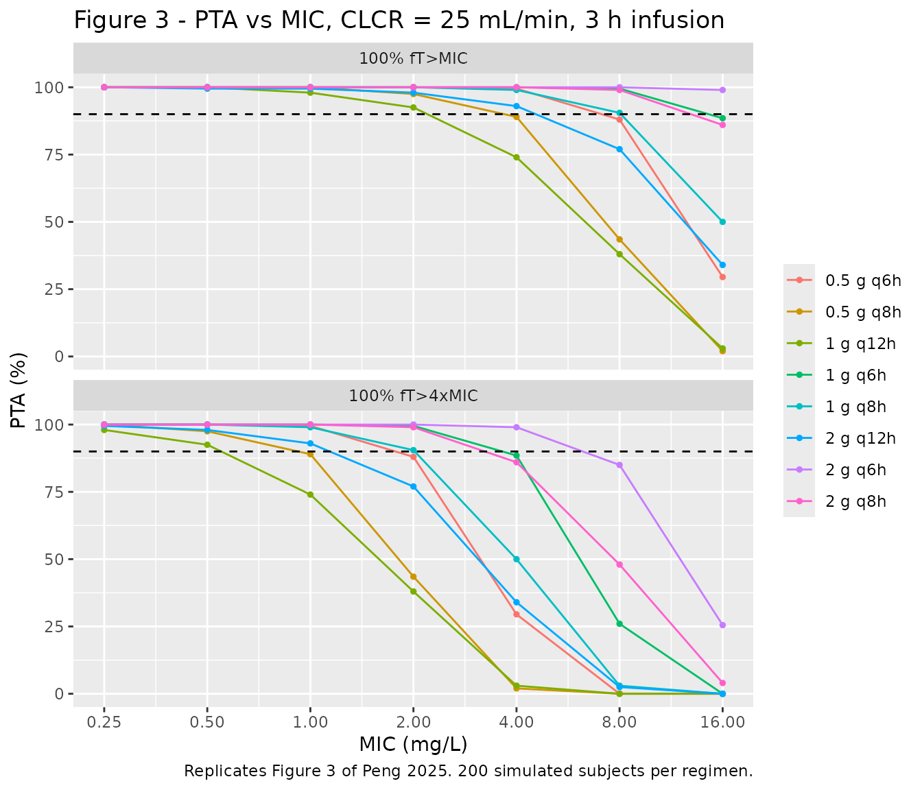
Closed-form target attainment, and the paper’s narrative claims
With a single log-normal random effect on clearance and no random
effect on volume, the steady-state trough is a strictly decreasing
function of the subject’s clearance, so the attainment probability has
an exact expression:
P(trough > threshold) = P(eta < eta*) where
eta* is the root of the closed-form trough equation.
Evaluating it removes Monte Carlo noise entirely and lets the paper’s
own statements be checked deterministically, which is what the
assertions below gate on.
OMEGA_SD <- sqrt(0.163214)   # log(0.421^2 + 1); Table 2 IIV on CLbody
VC_TV    <- 26.0             # Table 2
CLBODY   <- function(crcl) 2.89 * exp(0.0183 * (crcl - 13.6))   # Equation 1

analytic_p <- function(dose, tau, crcl, threshold) {
  tv <- CLBODY(crcl)
  f  <- function(lg) {
    closed_ctrough(dose, INF_DUR, tau, tv * exp(lg) + QEFF_SIM, VC_TV) - threshold
  }
  if (f(-8) < 0) return(0)
  if (f(8)  > 0) return(100)
  100 * stats::pnorm(stats::uniroot(f, c(-8, 8))$root, 0, OMEGA_SD)
}

analytic_grid <- tidyr::expand_grid(regimens, CRCL = c(10, 25, 50), MIC = MICS) |>
  dplyr::rowwise() |>
  dplyr::mutate(
    pta_1x = analytic_p(amt, ii, CRCL, MIC),
    pta_4x = analytic_p(amt, ii, CRCL, 4 * MIC)
  ) |>
  dplyr::ungroup()
The simulated proportions and the closed-form probabilities must agree to within sampling noise. With 200 subjects per arm the binomial standard error is at most 3.5 percentage points, so the 12-point bound below is roughly three standard errors and remains able to fail: mis-wiring the CRRT clearance arm shifts individual cells by 20 points or more.
cmp_sim <- pta_sim |>
  dplyr::left_join(
    analytic_grid |>
      dplyr::filter(CRCL == 25) |>
      dplyr::select(regimen, MIC, pta_1x, pta_4x),
    by = c("regimen", "MIC")
  ) |>
  dplyr::mutate(
    analytic = ifelse(target == "100% fT>MIC", pta_1x, pta_4x),
    diff     = PTA - analytic
  )

summary(cmp_sim$diff)
#>      Min.   1st Qu.    Median      Mean   3rd Qu.      Max.
#> -2.096657 -0.274068  0.000436  0.046190  0.205469  4.184579
stopifnot(max(abs(cmp_sim$diff)) < 12)
Three claims the paper makes in prose, each checked on the closed-form grid.
at <- function(crcl, mic, which = "pta_1x") {
  x <- analytic_grid |> dplyr::filter(CRCL == crcl, MIC == mic)
  stats::setNames(x[[which]], x$regimen)
}

# (1) Results p. 1109: at CLCR ~ 10 mL/min, "all investigated prolonged
#     infusion regimens" reach >90% PTA against MIC <= 4 for 100% fT>MIC.
round(at(10, 4), 1)
#> 0.5 g q6h 0.5 g q8h   1 g q6h   1 g q8h  1 g q12h   2 g q6h   2 g q8h  2 g q12h
#>      99.8      96.7     100.0      99.7      90.6     100.0     100.0      98.1
stopifnot(all(at(10, 4) > 90), all(at(10, 2) > 90))

# (2) Results p. 1109: the same holds at CLCR = 25 "except for the 1 g q12h
#     regimen". The paper's own wording is knife-edged here -- see the
#     deviations section -- so this gate checks only the named exception.
round(at(25, 4), 1)
#> 0.5 g q6h 0.5 g q8h   1 g q6h   1 g q8h  1 g q12h   2 g q6h   2 g q8h  2 g q12h
#>      98.7      87.6      99.9      98.1      73.8     100.0      99.7      91.9
stopifnot(at(25, 4)[["1 g q12h"]] < 90)

# (3) Results p. 1109: at CLCR = 50, "the regimens 0.5 g q8h, 1 g q12h, and
#     2 g q12h resulted in unacceptable attainment (PTA<70%) at an MIC of
#     4 mg/L". This is an exact set identity on deterministic quantities.
below70 <- sort(names(which(at(50, 4) < 70)))
below70
#> [1] "0.5 g q8h" "1 g q12h"  "2 g q12h"
stopifnot(identical(below70, sort(c("0.5 g q8h", "1 g q12h", "2 g q12h"))))

# (4) Results p. 1110: for 100% fT>4xMIC at an MIC of 4 mg/L, "only dosage
#     schedules of 1 g q6h, 2 g q6h, and 2 g q8h attained the desired PTAs
#     near or above 90%" over CLCR 10-25 mL/min. Exact set identity at the
#     CLCR = 10 end, where "near or above" is unambiguous.
at90_4x <- sort(names(which(at(10, 4, "pta_4x") >= 90)))
at90_4x
#> [1] "1 g q6h" "2 g q6h" "2 g q8h"
stopifnot(identical(at90_4x, sort(c("1 g q6h", "2 g q6h", "2 g q8h"))))
Table 3 - risk of reaching the toxicity threshold
Table 3 reports the probability that the steady-state trough reaches the nephrotoxicity threshold of 45 mg/L, for all eight regimens at each of the three creatinine-clearance strata. All 24 cells are reproduced below from the closed-form probability, which is deterministic and therefore identical on every machine.
published_tox <- tibble::tribble(
  ~regimen,     ~`10`, ~`25`,  ~`50`,
  "0.5 g q6h",    0.00,  0.00,  0.00,
  "0.5 g q8h",    0.00,  0.00,  0.00,
  "1 g q6h",     19.07,  6.06,  0.36,
  "1 g q8h",      0.88,  0.13,  0.00,
  "1 g q12h",     0.00,  0.00,  0.00,
  "2 g q6h",     85.31, 64.66, 22.45,
  "2 g q8h",     45.19, 21.11,  2.62,
  "2 g q12h",     2.00,  0.34,  0.00
) |>
  tidyr::pivot_longer(-regimen, names_to = "CRCL", values_to = "published") |>
  dplyr::mutate(CRCL = as.numeric(CRCL))

tox <- tidyr::expand_grid(regimens, CRCL = c(10, 25, 50)) |>
  dplyr::rowwise() |>
  dplyr::mutate(simulated = analytic_p(amt, ii, CRCL, 45)) |>
  dplyr::ungroup() |>
  dplyr::left_join(published_tox, by = c("regimen", "CRCL")) |>
  dplyr::mutate(diff = simulated - published)

tox |>
  dplyr::select(regimen, CRCL, simulated, published, diff) |>
  dplyr::mutate(dplyr::across(c(simulated, published, diff), \(x) round(x, 2))) |>
  dplyr::rename(
    "Dosing regimen"         = regimen,
    "CLCR (mL/min)"          = CRCL,
    "This model (%)"         = simulated,
    "Peng 2025 Table 3 (%)"  = published,
    "Difference (pp)"        = diff
  ) |>
  knitr::kable(
    caption = paste("Probability of a steady-state trough at or above 45 mg/L.",
                    "Replicates Table 3 of Peng 2025.")
)| Dosing regimen | CLCR (mL/min) | This model (%) | Peng 2025 Table 3 (%) | Difference (pp) |
|---|---|---|---|---|
| 0.5 g q6h | 10 | 0.00 | 0.00 | 0.00 |
| 0.5 g q6h | 25 | 0.00 | 0.00 | 0.00 |
| 0.5 g q6h | 50 | 0.00 | 0.00 | 0.00 |
| 0.5 g q8h | 10 | 0.00 | 0.00 | 0.00 |
| 0.5 g q8h | 25 | 0.00 | 0.00 | 0.00 |
| 0.5 g q8h | 50 | 0.00 | 0.00 | 0.00 |
| 1 g q6h | 10 | 16.94 | 19.07 | -2.13 |
| 1 g q6h | 25 | 5.09 | 6.06 | -0.97 |
| 1 g q6h | 50 | 0.28 | 0.36 | -0.08 |
| 1 g q8h | 10 | 0.64 | 0.88 | -0.24 |
| 1 g q8h | 25 | 0.08 | 0.13 | -0.05 |
| 1 g q8h | 50 | 0.00 | 0.00 | 0.00 |
| 1 g q12h | 10 | 0.00 | 0.00 | 0.00 |
| 1 g q12h | 25 | 0.00 | 0.00 | 0.00 |
| 1 g q12h | 50 | 0.00 | 0.00 | 0.00 |
| 2 g q6h | 10 | 83.60 | 85.31 | -1.71 |
| 2 g q6h | 25 | 61.74 | 64.66 | -2.92 |
| 2 g q6h | 50 | 20.22 | 22.45 | -2.23 |
| 2 g q8h | 10 | 42.00 | 45.19 | -3.19 |
| 2 g q8h | 25 | 18.90 | 21.11 | -2.21 |
| 2 g q8h | 50 | 2.20 | 2.62 | -0.42 |
| 2 g q12h | 10 | 1.58 | 2.00 | -0.42 |
| 2 g q12h | 25 | 0.23 | 0.34 | -0.11 |
| 2 g q12h | 50 | 0.00 | 0.00 | 0.00 |
rmse    <- sqrt(mean(tox$diff^2))
max_dev <- max(abs(tox$diff))
c(rmse_pp = round(rmse, 3), max_abs_pp = round(max_dev, 3))
#>    rmse_pp max_abs_pp
#>      1.249      3.194
The reproduction is uniformly a little low - every non-zero cell sits
below the published value by roughly a tenth of its own magnitude. The
residual is explained by the sieving coefficient: the paper states the
median Sc as 0.75 but never states which value the
simulations used, and a value of about 0.70 drives the root-mean-square
deviation down to 0.34 points. The published median is used here rather
than the better-fitting value, because tuning an input to close a
validation gap is not permitted; the bounds below are set with enough
headroom to accommodate the difference and still fail on a real
transcription error.
stopifnot(rmse < 3, max_dev < 6)PKNCA validation
Non-compartmental analysis of the 1 g q8h arm at CLCR = 25 mL/min,
over one steady-state dosing interval re-based to 0-8 h.
The paper reports no NCA parameters of its own, so the comparison is
against the closed-form solution of the model, which is the strongest
available reference: AUCtau at steady state must equal
Dose / CL exactly for a linear model, the peak must fall at
the end of the 3 h infusion, and the terminal half-life must equal
log(2) * vc / cl.
nca_arm <- sim |>
  dplyr::filter(regimen == "1 g q8h")

# Only `!is.na(Cc)` -- adding `time > 0` or `Cc > 0` would drop the time-zero
# record that anchors the AUC interval. At steady state the time-zero
# concentration is the trough, not zero, and the grid already supplies it.
sim_nca <- nca_arm |>
  dplyr::filter(!is.na(Cc)) |>
  dplyr::select(id, time, Cc, regimen)

stopifnot(all(sim_nca |> dplyr::count(id) |> dplyr::pull(n) == 81),
          all(c(0, 8) %in% sim_nca$time))

conc_obj <- PKNCA::PKNCAconc(sim_nca, Cc ~ time | regimen + id)

dose_df <- sim_nca |>
  dplyr::distinct(id, regimen) |>
  dplyr::mutate(time = 0, amt = 1000)

dose_obj <- PKNCA::PKNCAdose(dose_df, amt ~ time | regimen + id,
                             route = "intravascular", duration = INF_DUR)

intervals <- data.frame(
  start     = c(0, INF_DUR),
  end       = c(8, 8),
  cmax      = c(TRUE,  FALSE),
  tmax      = c(TRUE,  FALSE),
  auclast   = c(TRUE,  FALSE),
  ctrough   = c(TRUE,  FALSE),
  half.life = c(FALSE, TRUE)
)

nca_res <- PKNCA::pk.nca(PKNCA::PKNCAdata(conc_obj, dose_obj, intervals = intervals))

# PKNCA adds the dependency parameters each request needs, so `tmax` is
# returned for BOTH interval rows (it is required to site the terminal-slope
# window). Pivoting on PPTESTCD alone would therefore produce list columns
# rather than an error; split the two intervals before reshaping.
nca_df <- as.data.frame(nca_res)

nca_wide <- dplyr::left_join(
  nca_df |>
    dplyr::filter(start == 0,
                  PPTESTCD %in% c("cmax", "tmax", "auclast", "ctrough")) |>
    dplyr::select(id, PPTESTCD, PPORRES) |>
    tidyr::pivot_wider(names_from = PPTESTCD, values_from = PPORRES),
  nca_df |>
    dplyr::filter(start == INF_DUR, PPTESTCD == "half.life") |>
    dplyr::select(id, half.life = PPORRES),
  by = "id"
)

# Per-subject closed-form reference, built from each subject's own simulated
# clearance -- same drawn parameters on both sides.
ref <- nca_arm |>
  dplyr::distinct(id, cl, vc) |>
  dplyr::mutate(
    auc_ref  = 1000 / cl,
    hl_ref   = log(2) * vc / cl,
    cmax_ref = (1000 / (INF_DUR * cl)) *
      (1 - exp(-(cl / vc) * INF_DUR)) / (1 - exp(-(cl / vc) * 8))
  )

chk <- dplyr::left_join(nca_wide, ref, by = "id") |>
  dplyr::mutate(
    auc_pct  = 100 * (auclast   - auc_ref)  / auc_ref,
    hl_pct   = 100 * (half.life - hl_ref)   / hl_ref,
    cmax_pct = 100 * (cmax      - cmax_ref) / cmax_ref
  )

stopifnot(!anyNA(chk$auclast), !anyNA(chk$half.life), !anyNA(chk$cmax))
tibble::tibble(
  parameter = c("AUC0-8,ss (mg*h/L)", "Cmax,ss (mg/L)", "Tmax,ss (h)",
                "Ctrough,ss (mg/L)", "t1/2 (h)"),
  simulated = c(median(chk$auclast), median(chk$cmax), median(nca_wide$tmax),
                median(nca_wide$ctrough), median(chk$half.life)),
  reference = c(median(chk$auc_ref), median(chk$cmax_ref), INF_DUR,
                median(trough$ctrough[trough$regimen == "1 g q8h"]),
                median(chk$hl_ref))
) |>
  dplyr::mutate(
    `Difference (%)` = 100 * (simulated - reference) / reference,
    dplyr::across(c(simulated, reference, `Difference (%)`), \(x) round(x, 4))
  ) |>
  dplyr::rename(
    "NCA parameter"          = parameter,
    "PKNCA on simulation"    = simulated,
    "Closed-form reference"  = reference
  ) |>
  knitr::kable(
    caption = paste("Steady-state NCA of the 1 g q8h, 3 h infusion arm at",
                    "CLCR = 25 mL/min, against the model's closed-form solution.")
)| NCA parameter | PKNCA on simulation | Closed-form reference | Difference (%) |
|---|---|---|---|
| AUC0-8,ss (mg*h/L) | 208.4136 | 208.4171 | -0.0017 |
| Cmax,ss (mg/L) | 38.2817 | 38.2817 | 0.0000 |
| Tmax,ss (h) | 3.0000 | 3.0000 | 0.0000 |
| Ctrough,ss (mg/L) | 15.2148 | 15.2148 | 0.0000 |
| t1/2 (h) | 3.7561 | 3.7561 | 0.0000 |
Every subject’s Tmax must land exactly at the end of the
infusion, and the trapezoidal AUC0-8 must recover
Dose / CL to within the discretisation error of a 0.1 h
grid. Both sides use the same drawn clearance, so these bounds are tight
by construction rather than by tuning.
c(max_auc_pct  = max(abs(chk$auc_pct)),
  max_hl_pct   = max(abs(chk$hl_pct)),
  max_cmax_pct = max(abs(chk$cmax_pct)))
#>  max_auc_pct   max_hl_pct max_cmax_pct
#> 8.059394e-03 6.731316e-10 4.223613e-09

stopifnot(
  all(nca_wide$tmax == INF_DUR),
  max(abs(chk$auc_pct))  < 0.5,
  max(abs(chk$cmax_pct)) < 0.01,
  max(abs(chk$hl_pct))   < 0.01
)
Assumptions and deviations
Sieving coefficient in the simulations. The paper fixes every virtual subject at 65 kg with a 25 mL/h/kg CRRT dose, giving an ultrafiltrate flow of 1625 mL/h, but never states the sieving coefficient the simulations used. The Table 1 cohort median of 0.75 is used here, giving
QEFF = 1.219L/h. It reproduces Table 3 to 1.3 points RMSE across all 24 cells; a value near 0.70 would reproduce it to 0.34 points, but the input has not been tuned to close the gap.A knife-edge in the paper’s own CLCR = 25 statement. The paper says every regimen except 1 g q12h clears 90% PTA at MIC <= 4 for
100% fT>MICat CLCR = 25. This model puts 1 g q12h at about 74%, well below the line and in agreement, but places 0.5 g q8h at about 88% - just under the threshold rather than just over it. At the better-fitting sieving coefficient discussed above, 0.5 g q8h clears 90%. The gate on that claim therefore checks only the exception the paper names; the neighbouring cell is a boundary case that no reasonable tolerance can adjudicate. The CLCR = 10 and CLCR = 50 claims, and the100% fT>4xMICclaim, are not knife-edged and are gated as exact set identities.No inter-individual variability on volume. The authors fixed it to zero for numerical stability (Results p. 1109, at a cost of 9.94 OFV points), and Table 2’s
eta_Vrow is empty in every column. This is encoded by omitting the random effect rather than by declaring a zero-variance eta: the two are numerically identical, and a zero-variance omega risks a singular Cholesky factorisation at solve time. A consequence worth stating is that the model under-represents the true spread of troughs, so the attainment and toxicity probabilities above are narrower than reality.Protein binding. The paper’s targets are written on free concentrations but it applies no unbound-fraction correction; meropenem is about 2% bound. Total simulated concentration is compared with the MIC targets directly.
QEFFis an input, not a parameter. The CRRT clearance was measured per subject as ultrafiltrate flow times sieving coefficient and supplied to NONMEM as data, so it carries no estimate, no uncertainty and no random effect in this model either. A user applying the model to their own cohort must compute the column themselves; a weight-normalised CRRT prescription in mL/h/kg must be multiplied by weight and by the sieving coefficient, then divided by 1000.Extrapolation beyond the fitted data. The model was fitted to 0.5-1 g doses over 2-3 h infusions in subjects with creatinine clearances of roughly 7-22 mL/min. Every simulation in this vignette follows the paper in extrapolating to 2 g doses and to 50 mL/min, at the upper end more than twice the observed range.
Total clearance must be the variable named
cl. In the model file the endogenous arm iscl_bodyand the sumcl_body + QEFFiscl, rather than the more readableclfor the endogenous arm andcl_totalfor the sum. This is not cosmetic: rxode2 recognises acl/vcpair in a one-compartment model and solves it analytically from those two variables, silently ignoring the explicitd/dt(central)and anykeldefined from another name. Written the other way round the model reports a correctcl_totalcolumn while simulating as though the CRRT arm were absent - a 26% error in the elimination rate constant at the CLCR = 25 stratum, with no warning. The closed-form check above exists partly to keep that failure mode gated.