Cefiderocol (Sanz-Codina 2024)
Source:vignettes/articles/SanzCodina_2024_cefiderocol.Rmd
SanzCodina_2024_cefiderocol.RmdModel and source
- Citation: Sanz-Codina M, van Os W, Pham AD, Jorda A, Wolf-Duchek M, Bergmann F, Lackner E, Lier C, van Hasselt JGC, Minichmayr IK, Dorn C, Zeitlinger M, al Jalali V. Target-site cefiderocol pharmacokinetics in soft tissues of healthy volunteers. J Antimicrob Chemother. 2024;79(12):3281. doi:10.1093/jac/dkae359. PMID 39373642; PMCID PMC11638555.
- Description: Two-compartment population PK model for intravenous cefiderocol in healthy adult male volunteers, fitted to total and unbound plasma concentrations and to microdialysis-derived unbound interstitial concentrations in subcutaneous adipose and skeletal muscle tissue (Sanz-Codina 2024). Clearance and volumes are referenced to the UNBOUND concentration; total plasma cefiderocol is Cunbound / fu with a constant estimated fraction unbound, and each tissue concentration is the peripheral-compartment concentration multiplied by a tissue scaling factor.
- Article: https://doi.org/10.1093/jac/dkae359 (open access, PMC11638555)
Sanz-Codina and colleagues gave eight healthy men a single 2 g
intravenous dose of cefiderocol over 3 h and measured total plasma
concentrations, unbound plasma concentrations (ultrafiltration at 3, 4
and 7 h) and unbound interstitial concentrations in subcutaneous adipose
and skeletal muscle tissue by microdialysis. The final population model
is a two-compartment model fitted to UNBOUND concentrations with a
constant estimated fraction unbound (fu); the two tissue
concentrations are the peripheral-compartment concentration multiplied
by a tissue scaling factor (TFsub, TFmus).
Population
Eight healthy male volunteers aged 18-55 years (mean 34.9 +/- 8.9 years) with body mass index 19-30 kg/m^2 (mean 24.6 +/- 1.1 kg/m^2) and a Cockcroft-Gault creatinine clearance above 90 mL/min, studied at the Medical University of Vienna (Methods, “Study population and in vivo procedures”; Results, “Study population and safety”). Race was not reported. The model has no covariates: the authors state that the small, homogeneous cohort precluded a covariate analysis.
The same information is available programmatically via
readModelDb("SanzCodina_2024_cefiderocol")()$population.
Source trace
| Equation / parameter | Value | Source location |
|---|---|---|
lcl (CL, unbound-referenced) |
log(11.0) L/h | Table 2, ‘CL (L/h)’ |
lvc (Vc, unbound-referenced) |
log(11.3) L | Table 2, ‘Vc (L)’ |
lq (Q12) |
log(25.3) L/h | Table 2, ‘Q12 (L/h)’ |
lvp (Vp) |
log(15.1) L | Table 2, ‘Vp (L)’ |
lfu (fraction unbound) |
log(0.639) | Table 2, ‘fu’ |
lkp_adipose (TFsub) |
log(0.943) | Table 2, ‘TFsub’ |
lkp_muscle (TFmus) |
log(0.901) | Table 2, ‘TFmus’ |
etalcl |
0.0298 (17.4% CV) | Table 2, IIV ‘CL (CV%)’; omega^2 = log(CV^2 + 1) per Table 2 footnote |
etalvc |
0.0679 (26.5% CV) | Table 2, IIV ‘Vc (CV%)’ |
etalkp_adipose |
0.0755 (28.0% CV) | Table 2, IIV ‘TFsub (CV%)’ |
etalkp_muscle |
0.0616 (25.2% CV) | Table 2, IIV ‘TFmus (CV%)’ |
propSd, propSd_Cunbound
|
0.0585 | Table 2, ‘Propplasma (CV%)’ = 5.85 (one plasma error) |
propSd_Cadipose, propSd_Cmuscle
|
0.303 | Table 2, ‘Proptissue (CV%)’ = 30.3 (one tissue error) |
addSd_Cadipose, addSd_Cmuscle
|
2.3 mg/L | Table 2, ‘Addtissue (mg/L)’ = 2.3 |
| Two-compartment structure, first-order elimination | n/a | Methods ‘Population PK analysis’; Results ‘Population PK model and PTA analysis’ |
Cunbound = central / vc;
Cc = Cunbound / fu
|
n/a | Table 2 footnote (‘Estimates are based on unbound cefiderocol concentrations’); Methods (fu estimated from total vs unbound) |
Cadipose, Cmuscle = TF x
peripheral1 / vp
|
n/a | Results: tissue concentrations scaled to the peripheral compartment |
Virtual cohort
The observed data are not public. A virtual cohort of 200 subjects
(the trial had 8) receives the trial regimen, 2 g over 3 h. Random
effects are drawn in base R from the model’s omega matrix and passed to
a typical-value solve through params, so the cohort depends
only on set.seed() and is identical on every machine.
mod <- readModelDb("SanzCodina_2024_cefiderocol")
ui <- rxode2::rxode2(mod)
#> ℹ parameter labels from comments will be replaced by 'label()'

set.seed(20241211)
n_sub <- 200L
omega <- ui$omega
eta <- matrix(rnorm(n_sub * nrow(omega)), n_sub) %*% chol(omega)
colnames(eta) <- rownames(omega)
params <- data.frame(id = seq_len(n_sub), eta)

# All four endpoints are algebraic observables, so observation rows are keyed
# by dvid with an empty cmt; doses go to the central ODE state.
make_events <- function(ids, dose_times, obs_times, dose = 2000, dur = 3) {
  doses <- tidyr::expand_grid(id = ids, time = dose_times) |>
    dplyr::mutate(
      amt = dose,
      rate = dose / dur,
      evid = 1L,
      cmt = "central",
      dvid = NA_integer_
    )
  obs <- tidyr::expand_grid(id = ids, time = obs_times) |>
    dplyr::mutate(amt = 0, rate = 0, evid = 0L, cmt = NA_character_, dvid = 1L)
  dplyr::bind_rows(doses, obs) |>
    dplyr::arrange(id, time, dplyr::desc(evid))
}

events_sd <- make_events(params$id, dose_times = 0, obs_times = seq(0, 8, by = 0.1))
stopifnot(!anyDuplicated(events_sd[, c("id", "time", "evid")]))
Simulation
sim_sd <- rxode2::rxSolve(
  rxode2::zeroRe(mod),
  events = events_sd,
  params = params,
  useLinCmt = FALSE
) |>
  as.data.frame() |>
  dplyr::distinct(id, time, .keep_all = TRUE)
#> ℹ parameter labels from comments will be replaced by 'label()'
#> Warning: multi-subject simulation without without 'omega'

stopifnot(nrow(sim_sd) == n_sub * length(seq(0, 8, by = 0.1)))
stopifnot(!anyNA(sim_sd[, c("Cc", "Cunbound", "Cadipose", "Cmuscle")]))
Replicate published figures
Figure 2: visual predictive check
Residual error is added in base R with the Table 2 magnitudes (proportional for both plasma outputs, combined proportional + additive for the tissues) so the bands are comparable to the VPC. The dashed lines are the 10th and 90th percentiles and the solid line the median, as in the paper.
th <- ui$theta
long_sd <- sim_sd |>
  dplyr::select(id, time, Cc, Cunbound, Cadipose, Cmuscle) |>
  tidyr::pivot_longer(-c(id, time), names_to = "output", values_to = "ipred")

set.seed(7)
eps1 <- rnorm(nrow(long_sd))
long_sd <- long_sd |>
  dplyr::mutate(
    prop = dplyr::case_when(
      output == "Cc" ~ th[["propSd"]],
      output == "Cunbound" ~ th[["propSd_Cunbound"]],
      output == "Cadipose" ~ th[["propSd_Cadipose"]],
      output == "Cmuscle" ~ th[["propSd_Cmuscle"]]
    ),
    add = dplyr::case_when(
      output == "Cadipose" ~ th[["addSd_Cadipose"]],
      output == "Cmuscle" ~ th[["addSd_Cmuscle"]],
      TRUE ~ 0
    ),
    # nlmixr2 combined2: variance = add^2 + (prop * ipred)^2
    dv = ipred + sqrt(add^2 + (prop * ipred)^2) * eps1
  )

panel_labels <- c(
  Cc = "Plasma (total)",
  Cunbound = "Plasma (free)",
  Cadipose = "Subcutis (free)",
  Cmuscle = "Muscle (free)"
)

long_sd |>
  dplyr::filter(time >= 1) |>
  dplyr::group_by(output, time) |>
  dplyr::summarise(
    p10 = quantile(dv, 0.10),
    p50 = quantile(dv, 0.50),
    p90 = quantile(dv, 0.90),
    .groups = "drop"
  ) |>
  dplyr::mutate(output = factor(panel_labels[output], levels = panel_labels)) |>
  ggplot(aes(time, p50)) +
  geom_ribbon(aes(ymin = p10, ymax = p90), alpha = 0.2) +
  geom_line() +
  geom_line(aes(y = p10), linetype = "dashed") +
  geom_line(aes(y = p90), linetype = "dashed") +
  facet_wrap(~output, nrow = 1) +
  labs(
    x = "Time (h)",
    y = "Cefiderocol (mg/L)",
    caption = "Replicates Figure 2 of Sanz-Codina 2024 (simulated 10th/50th/90th percentiles)."
  )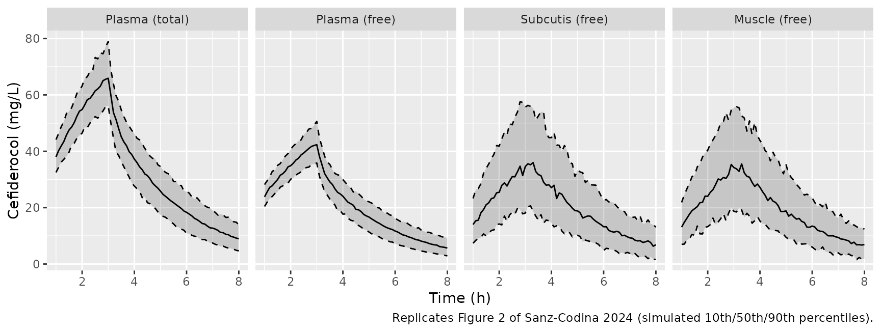
The shapes match Figure 2: total plasma peaks at the end of the 3 h infusion (typical-value prediction about 67 mg/L), unbound plasma is about 64% of total, and the two tissue curves rise more slowly and peak just after the end of infusion at roughly 35 mg/L (typical value). The 10th-90th percentile band is wide in tissue because of the large tissue residual error.
PKNCA validation
PKNCA is run on the individual predictions (no residual error) of each unbound output over 0-8 h, matching the non-compartmental analysis of Table 1.
nca_in <- long_sd |>
  dplyr::filter(output %in% c("Cunbound", "Cadipose", "Cmuscle"), !is.na(ipred)) |>
  dplyr::transmute(
    id,
    time,
    Cc = ipred,
    output = unname(panel_labels[output])
  )

# The solve includes a time-zero observation for every subject; assert it so a
# change to the grid cannot silently drop the AUC anchor.
stopifnot(all(dplyr::summarise(nca_in, t0 = any(time == 0), .by = c(id, output))$t0))

dose_in <- tidyr::expand_grid(id = params$id, output = unique(nca_in$output)) |>
  dplyr::mutate(time = 0, amt = 2000)

conc_obj <- PKNCA::PKNCAconc(nca_in, Cc ~ time | output + id)
dose_obj <- PKNCA::PKNCAdose(dose_in, amt ~ time | output + id)
intervals <- data.frame(
  start = 0,
  end = 8,
  cmax = TRUE,
  auclast = TRUE,
  half.life = TRUE
)
nca_res <- PKNCA::pk.nca(PKNCA::PKNCAdata(conc_obj, dose_obj, intervals = intervals))
Comparison against published NCA
Table 1 reports arithmetic means, so the simulated per-subject values are summarised by their mean before the comparison.
sim_mean <- as.data.frame(nca_res) |>
  dplyr::filter(PPTESTCD %in% c("cmax", "auclast", "half.life")) |>
  dplyr::summarise(PPORRES = mean(PPORRES, na.rm = TRUE), .by = c(output, PPTESTCD))

published <- tibble::tribble(
  ~output,           ~half.life, ~cmax, ~auclast,
  "Subcutis (free)", 1.82,       41.6,  163.2,
  "Muscle (free)",   1.30,       40.9,  151.7,
  "Plasma (free)",   2.04,       39.9,  162.0
)

cmp <- nlmixr2lib::ncaComparisonTable(
  simulated = sim_mean,
  reference = published,
  by = "output",
  units = c(cmax = "mg/L", auclast = "h*mg/L, 0-8 h", half.life = "h"),
  tolerance_pct = 20
)
knitr::kable(cmp, caption = "Simulated vs. Table 1 NCA (means). * differs by >20%.")| NCA parameter | output | Reference | Simulated | % diff |
|---|---|---|---|---|
| Cmax (mg/L) | Subcutis (free) | 41.6 | 37.2 | -10.5% |
| Cmax (mg/L) | Muscle (free) | 40.9 | 35.9 | -12.1% |
| Cmax (mg/L) | Plasma (free) | 39.9 | 42.7 | +7.0% |
| AUClast (h*mg/L, 0-8 h) | Subcutis (free) | 163 | 157 | -3.9% |
| AUClast (h*mg/L, 0-8 h) | Muscle (free) | 152 | 151 | -0.2% |
| AUClast (h*mg/L, 0-8 h) | Plasma (free) | 162 | 166 | +2.2% |
| t½ (h) | Subcutis (free) | 1.82 | 1.97 | +8.0% |
| t½ (h) | Muscle (free) | 1.3 | 1.97 | +51.2%* |
| t½ (h) | Plasma (free) | 2.04 | 1.95 | -4.6% |
auc_mean <- sim_mean |>
  dplyr::filter(PPTESTCD == "auclast") |>
  dplyr::left_join(
    dplyr::select(published, output, ref = auclast),
    by = "output"
  ) |>
  dplyr::mutate(pct = 100 * (PPORRES / ref - 1))
stopifnot(nrow(auc_mean) == 3L)
# Unbound AUC0-8 is the quantity the model was built to reproduce; a wrong CL,
# volume, fu or scaling factor moves it by tens of percent.
stopifnot(all(abs(auc_mean$pct) < 15))
The unbound AUC0-8 in plasma and both tissues is within 4% of Table 1, and Cmax within 12%. The simulated tissue Cmax is about 10% below the observed mean; an observed Cmax is the largest of several noisy microdialysate values (tissue residual error about 30%), which biases it upward relative to the maximum of a smooth individual prediction. The one starred row is the muscle half-life: Table 1 gives 1.30 h from the observed microdialysis curves, whereas in the model every tissue concentration is a constant multiple of the peripheral compartment and therefore shares the plasma terminal half-life (about 2 h). The paper notes that the model did not fully capture the shape of the muscle profile (a possible delay in distribution to muscle).
Probability of target attainment (Figure 3)
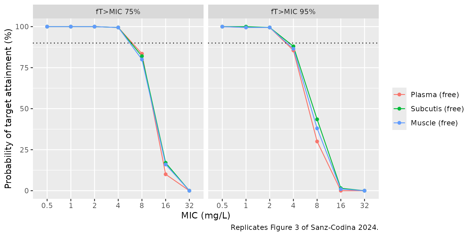
The paper simulated the first 24 h of 2 g every 8 h, each dose infused over 3 h, and computed the percentage of 0-24 h with the unbound concentration above the MIC in plasma, subcutis and muscle. The same 200-subject cohort is used here, on individual predictions.
events_md <- make_events(
  params$id,
  dose_times = c(0, 8, 16),
  obs_times = seq(0, 24, by = 0.05)
)
sim_md <- rxode2::rxSolve(
  rxode2::zeroRe(mod),
  events = events_md,
  params = params,
  useLinCmt = FALSE
) |>
  as.data.frame() |>
  dplyr::distinct(id, time, .keep_all = TRUE)
#> ℹ parameter labels from comments will be replaced by 'label()'
#> Warning: multi-subject simulation without without 'omega'
stopifnot(!anyNA(sim_md[, c("Cunbound", "Cadipose", "Cmuscle")]))

mics <- c(0.5, 1, 2, 4, 8, 16, 32)
ft_above <- sim_md |>
  dplyr::filter(time < 24) |>
  dplyr::select(id, Cunbound, Cadipose, Cmuscle) |>
  tidyr::pivot_longer(-id, names_to = "output", values_to = "conc") |>
  tidyr::expand_grid(mic = mics) |>
  dplyr::summarise(ft = 100 * mean(conc > mic), .by = c(id, output, mic))

pta <- tidyr::expand_grid(target = c(75, 95), ft_above) |>
  dplyr::summarise(pta = 100 * mean(ft >= target), .by = c(target, output, mic)) |>
  dplyr::mutate(output = factor(panel_labels[output], levels = panel_labels[-1]))

ggplot(pta, aes(factor(mic), pta, colour = output, group = output)) +
  geom_line() +
  geom_point() +
  geom_hline(yintercept = 90, linetype = "dotted") +
  facet_wrap(~target, labeller = labeller(target = function(x) paste0("fT>MIC ", x, "%"))) +
  labs(
    x = "MIC (mg/L)",
    y = "Probability of target attainment (%)",
    colour = NULL,
    caption = "Replicates Figure 3 of Sanz-Codina 2024."
  )
pta_cell <- function(tgt, out, m) {
  v <- pta$pta[pta$target == tgt & pta$output == out & pta$mic == m]
  if (length(v) != 1L) stop("no unique PTA row for ", tgt, "/", out, "/", m)
  v
}

pta |>
  dplyr::filter(mic %in% c(4, 8, 16)) |>
  tidyr::pivot_wider(names_from = mic, values_from = pta, names_prefix = "MIC ") |>
  dplyr::rename("fT>MIC target (%)" = target, "Matrix" = output) |>
knitr::kable(digits = 0, caption = "Simulated PTA (%) at MIC 4, 8 and 16 mg/L.")| fT>MIC target (%) | Matrix | MIC 4 | MIC 8 | MIC 16 |
|---|---|---|---|---|
| 75 | Plasma (free) | 100 | 84 | 10 |
| 75 | Subcutis (free) | 100 | 82 | 17 |
| 75 | Muscle (free) | 100 | 80 | 16 |
| 95 | Plasma (free) | 86 | 30 | 0 |
| 95 | Subcutis (free) | 88 | 44 | 2 |
| 95 | Muscle (free) | 86 | 38 | 1 |
# The paper's headline: PTA >= 90% up to MIC 4 mg/L in plasma and both tissues
# for the 75% target. The model-true values are ~99%, more than 10 binomial
# standard errors (n = 200) above the 90% line.
for (out in levels(pta$output)) stopifnot(pta_cell(75, out, 4) >= 90)
# Figure 3 shows PTA collapsing between 8 and 32 mg/L (fT>MIC 75%: ~11-18% at
# 16 mg/L; fT>MIC 95%: ~32-40% at 8 mg/L). Bounds sit several binomial
# standard errors wide of those values while still failing for a CL or
# volume off by 25%.
for (out in levels(pta$output)) {
  stopifnot(pta_cell(75, out, 16) < 45, pta_cell(75, out, 32) < 5)
  stopifnot(pta_cell(95, out, 8) > 10, pta_cell(95, out, 8) < 70)
}
The simulated curves reproduce Figure 3. For fT>MIC 75%, attainment is complete up to 4 mg/L and falls to about 80-85% at 8 mg/L and 10-17% at 16 mg/L (Figure 3: about 81-88% and 11-18%). For fT>MIC 95%, attainment at 4 mg/L is 86-88% against about 90-92% in Figure 3, and 30-44% at 8 mg/L (Figure 3: about 32-40%). Attainment is near zero at 32 mg/L in all three matrices. The shortfall of about 4 percentage points at 4 mg/L for the 95% target is under two binomial standard errors of a 200-subject cohort (about 2.4 points), and was not tuned.
Assumptions and deviations
-
Microdialysis observation model. The paper fitted
each recovery-corrected microdialysate concentration as the integral of
the tissue curve over its collection interval. The packaged
CadiposeandCmuscleare instantaneous unbound interstitial concentrations; to fit or compare against raw microdialysate data, average them over the collection interval. -
Shared residual errors. The paper estimated one
proportional error for plasma (total and unbound observations) and one
combined error for both tissues. nlmixr2 carries one error parameter per
endpoint, so the shared estimates are repeated (
propSd=propSd_Cunbound; the_Cadiposeand_Cmusclepairs are equal). Re-estimating the model would treat them as separate parameters. -
Combined error form. The paper does not say whether
the tissue combined error adds standard deviations or variances; the
nlmixr2 default (
combined2, variances add) is used. - IIV scale. Table 2 reports IIV as CV% computed from sqrt(exp(omega^2) - 1), so the variances are log(CV^2 + 1).
- PTA. The PTA simulation uses individual predictions without residual error and a 200-subject cohort (the paper used 5000 subjects); whether the paper’s PTA included residual error is not stated.
-
Naming. The tissue scaling factors TFsub and TFmus
are encoded as the partition-coefficient canonicals
lkp_adiposeandlkp_muscle; note that they scale the peripheral-compartment concentration, not the central plasma concentration. The subcutaneous microdialysis probe sampled subcutaneous adipose tissue, henceadipose. - No erratum or correction notice was found for this article (Europe PMC, checked 2026-10-31).