Clavulanic acid (Schouwenburg 2025)
Source:vignettes/articles/Schouwenburg_2025_clavulanicAcid.Rmd
Schouwenburg_2025_clavulanicAcid.RmdModel and source
Citation: Schouwenburg S, Keij FM, Tramper-Stranders GA, Kornelisse RF, Reiss IKM, De Cock PAJG, Dhont E, Watt KM, Muller AE, Flint RB, Koch BCP, Allegaert K, Preijers T. A Pooled Population Pharmacokinetic Study of Oral and Intravenous Administration of Clavulanic Acid in Neonates and Infants: Targeting Effective Beta-Lactamase Inhibition. Clin Pharmacol Ther. 2025;117(1):193-202. doi:10.1002/cpt.3423. The companion amoxicillin model this paper simulates alongside clavulanic acid (its reference 18) is available as modellib(‘Keij_2023_amoxicillin’).
Description: One-compartment population PK model with first-order absorption and estimated oral bioavailability for clavulanic acid in preterm and term neonates and infants up to 1 year of age, pooled from four datasets (RAIN, Staph Trio/Durham, De Cock, Dhont) covering both oral and intravenous amoxicillin/clavulanic acid and ticarcillin/clavulanic acid. Clearance carries a priori allometric weight scaling (fixed exponent 0.75, reference 3.9 kg) plus one estimated postnatal-age power term (reference 55.5 days); central volume carries fixed linear weight scaling (exponent 1, reference 3.9 kg). Oral bioavailability is 24.4%, estimated from neonates up to 10 days of age, and absorption is rapid (Ka 0.781 1/h). Interindividual variability is on clearance only; residual error is proportional (log-transform-both-sides, 77.8%) (Schouwenburg 2025).
Article: https://doi.org/10.1002/cpt.3423 (PMC11652805, open access)
Schouwenburg 2025 is the first population PK model for clavulanic acid in neonates and infants. It pools four datasets and describes both oral and intravenous clavulanic acid with a one-compartment model with first-order absorption and an estimated oral bioavailability.
The companion amoxicillin model that this paper simulates alongside
clavulanic acid (its reference 18, Keij 2023) is also packaged, as
modellib("Keij_2023_amoxicillin"). It is used further down
to reproduce the paper’s amoxicillin/clavulanic acid AUC-ratio
table.
Population
| Field | Value |
|---|---|
| species | human |
| n_subjects | 89 |
| n_studies | 4 |
| n_observations | 403 |
| age_range | postnatal age 0-365 days (pooled median 54.5 days) |
| ga_range | gestational age 23.0-41.7 weeks (pooled median 37.4 weeks) |
| pma_range | postmenstrual age 24.9-92.1 weeks (pooled median 45.1 weeks) |
| weight_range | 0.55-9.0 kg |
| weight_median | 3.9 kg |
| sex_female_pct | 32.2 |
| disease_state | preterm and term neonates and infants treated for probable, suspected or confirmed bacterial infection; includes critically ill children in paediatric and cardiac intensive care |
| dose_range | clavulanic acid 1.4-80 mg per administration (median 22 mg); 2.3-10.8 mg/kg/day (median 5.2); median 5 mg/kg/dose (range 1.0-12.8) |
| routes | oral (42 subjects, 82 concentrations) and intravenous (47 subjects, 321 concentrations); 6 of the 42 oral subjects switched from intravenous to oral during sampling |
| regions | The Netherlands (RAIN), Belgium (Ghent: De Cock and Dhont), USA (Durham/Staph Trio) |
| notes | Pooled analysis of four datasets (Schouwenburg 2025 Table 1): (1) RAIN (Reduction of intravenous Antibiotics In Neonates, The Netherlands), n = 42, oral and intravenous, PMA >= 35 weeks, PNA 0-28 days, weight >= 2 kg, amoxicillin/clavulanic acid 4:1; (2) Staph Trio / Durham (USA), n = 15, intravenous, PNA < 91 days, GA < 30 weeks, normal renal function, ticarcillin/clavulanic acid 30:1; (3) De Cock et al. (Ghent University Hospital paediatric ICU, Belgium), n = 6, intravenous, amoxicillin/clavulanic acid 5:1, restricted here to patients younger than 1 year; (4) Dhont et al. (Ghent cardiac ICU, Belgium, not yet published at time of writing), n = 26, intravenous, amoxicillin/clavulanic acid 5:1 and 10:1, critically ill children after cardiac surgery. Race/ethnicity was not reported. Modelling was in NONMEM 7.4.3 with PsN 4.2.0, Pirana 3.0.0 and R 4.1.2. Log-transform-both-sides was applied. 50 of 403 samples (12%) were below the lower limit of quantification (430 ng/mL = 0.43 mg/L per Figure 2) and were RETAINED and handled with Beal’s M3 method rather than excluded; M3 is an estimation-time likelihood method and has no simulation-time counterpart, so it is not encoded here. Free (unbound) concentrations were NOT measured: only total clavulanic acid concentrations were available, and the model was NOT corrected for protein binding. The authors note adult clavulanic acid protein binding is only moderate (up to 30%) and that neonates start with lower protein binding, so the paper’s %fT>CT target attainment is computed on total concentrations. Serum creatinine was available for every dataset EXCEPT the RAIN oral subjects and was therefore omitted from the covariate analysis entirely (Methods), which the authors flag as a possible source of unexplained clearance variability. Study centre was screened on clearance and not retained. Covariates screened and NOT retained: sex, gestational age, postmenstrual age, and study centre; only postnatal age was retained (dOFV -14.0, P < 0.05). Model evaluation was internal only (nonparametric bootstrap, n = 1000, of which 82.8% of runs were successful; GOF plots; VPC). No external validation was performed. Limited sampling in the oral subjects precluded estimation of interindividual variability on either bioavailability or Ka, so neither carries an eta. |
The cohort was 89 (pre)term neonates and infants (42 oral, 47
intravenous) contributing 403 plasma clavulanic acid concentrations,
pooled from four studies (Schouwenburg 2025 Table 1): RAIN (The
Netherlands, oral and intravenous, amoxicillin/clavulanic acid 4:1),
Staph Trio / Durham (USA, intravenous ticarcillin/clavulanic acid 30:1),
De Cock et al. (Ghent paediatric ICU, intravenous 5:1) and Dhont et
al. (Ghent cardiac ICU, intravenous 5:1 and 10:1). Median gestational
age was 37.4 weeks (range 23.0-41.7), median postnatal age 54.5 days
(0-365) and median current body weight 3.9 kg (0.55-9.0). The population
metadata is also available programmatically via
readModelDb("Schouwenburg_2025_clavulanicAcid")()$population.
Note that the oral sub-cohort that supports the bioavailability estimate is much narrower than the pooled cohort: RAIN only, postnatal age 0-12 days (median 2.9), weight 2.7-4.5 kg. The authors deliberately capped their own oral simulations at postnatal age 10 days “to prevent extrapolation of oral data”.
Source trace
The per-parameter origin is recorded as an in-file comment next to
each ini() entry in
inst/modeldb/specificDrugs/Schouwenburg_2025_clavulanicAcid.R.
The table below collects them in one place for review.
| Equation / parameter | Value | Source location |
|---|---|---|
lka (Ka) |
0.781 1/h (RSE 7%) | Table 2, “Ka (hour-1)”; bootstrap 0.801 (0.499-1.610). Restated in Discussion. |
lcl (TVCL) |
0.675 L/h (RSE 9%) | Table 2, “TVCL (L/h)”; bootstrap 0.685 (0.581-0.782). Restated in Discussion as 0.68. |
lvc (TVV) |
1.88 L (RSE 11%) | Table 2, “TVV (L)”; bootstrap 1.907 (1.558-2.274). |
lfdepot (F) |
0.244 (RSE 14%) | Table 2, “F (%)” = 24.4; bootstrap 24.7 (19-31.4). Abstract, Results, Discussion all say 24.4%. |
e_wt_cl |
0.75, fixed | Table 2 CL equation (BW/3.9)^0.75; Methods: “a priori
allometric scaling with a fixed exponent (i.e., 0.75 on clearances, 1 on
distribution volume)”. |
e_wt_vc |
1, fixed | Table 2 V equation TVV * (BW/3.9) (exponent implicit);
made explicit by the same Methods sentence. |
e_pna_cl (theta_PNA) |
0.207 (RSE 24%) | Table 2, “theta_PNA” under “Covariate relationships”; bootstrap 0.211 (0.124-0.290). Retained with dOFV -14.0, P < 0.05. |
etalcl |
omega^2 = 0.142129 (37.7 %CV) | Table 2, “Inter-individual variability (IIV) / Clearance (%CV)” = 37.7 (RSE 15%) [shrinkage 27%]; bootstrap 35.9 (24.5-46.0), a CV-scale interval. |
propSd |
0.778 | Table 2, “Proportional error (%)” = 77.8 (RSE 7%); bootstrap 77.5 (68.0-87.0). Methods and Table 2 footnote: log-transform both sides, log-scale additive error. |
| Reference weight 3.9 kg, reference PNA 55.5 d | n/a | Table 2 footnote: “Current bodyweight and postnatal age are scaled to the dataset median (3.9 kg and 55.5 days)”. |
CL = TVCL * (BW/3.9)^0.75 * (PNA/55.5)^theta_PNA |
n/a | Table 2, row “CLclav (L/hour)”. |
V = TVV * (BW/3.9) |
n/a | Table 2, row “Vclav (L)”. |
| One compartment, first-order absorption, estimated F | n/a | Results, “Final population pharmacokinetic model”. |
f(depot) <- exp(lfdepot), IV into
central
|
n/a | Table 1 route-of-administration row (RAIN oral and IV; others IV only). |
PNA is supplied in months (the
canonical nlmixr2lib unit) while the paper reports postnatal age in
days; model() therefore converts the
55.5-day reference once, as 55.5 / 30.4375 = 1.8234 months.
The ratio is unit-invariant, so theta_PNA transfers
unchanged. This follows the Zhao_2018_omeprazole and
Keij_2023_amoxicillin precedents.
Structural verification (closed-form gates)
Before any figure replication, the implementation is checked against identities the structural model must satisfy exactly. For a one-compartment model with first-order absorption these are analytic, so they are hard gates rather than eyeball comparisons.
d2m <- 30.4375  # days per month, for the PNA unit conversion

# Analytic parameters at an arbitrary covariate point
analytic <- function(WT, PNAd) {
  cl <- 0.675 * (WT / 3.9)^0.75 * (PNAd / 55.5)^0.207
  vc <- 1.88 * (WT / 3.9)
  list(cl = cl, vc = vc, kel = cl / vc, ka = 0.781, fdepot = 0.244)
}

# --- Gate 1: IV single dose, AUC(0-inf) must equal Dose / CL exactly
p <- analytic(WT = 3.9, PNAd = 55.5)
ev_iv <- rxode2::et(amt = 22, cmt = "central") |>
  rxode2::et(seq(0, 60, by = 0.005), cmt = "central")
ev_iv <- as.data.frame(ev_iv)
ev_iv$WT <- 3.9
ev_iv$PNA <- 55.5 / d2m
s_iv <- rxode2::rxSolve(ui, ev_iv, omega = NA, returnType = "data.frame")
trap <- function(t, y) sum(diff(t) * (head(y, -1) + tail(y, -1)) / 2)
s_iv_o <- dplyr::filter(s_iv, !is.na(Cc))
auc_iv <- trap(s_iv_o$time, s_iv_o$Cc)

# --- Gate 2: oral single dose, AUC(0-inf) must equal F * Dose / CL exactly
ev_or <- rxode2::et(amt = 27, cmt = "depot") |>
  rxode2::et(seq(0, 60, by = 0.005), cmt = "central")
ev_or <- as.data.frame(ev_or)
ev_or$WT <- 3.9
ev_or$PNA <- 55.5 / d2m
s_or <- rxode2::rxSolve(ui, ev_or, omega = NA, returnType = "data.frame") |>
  dplyr::filter(!is.na(Cc))
auc_or <- trap(s_or$time, s_or$Cc)

gates <- tibble::tibble(
  Gate = c("IV AUC(0-inf) = Dose/CL",
           "Oral AUC(0-inf) = F*Dose/CL",
           "Terminal half-life = log(2)/kel",
           "Solved CL at reference = TVCL",
           "Solved V at reference = TVV"),
  Analytic = c(22 / p$cl,
               p$fdepot * 27 / p$cl,
               log(2) / p$kel,
               0.675,
               1.88),
  Simulated = c(auc_iv,
                auc_or,
                {
                  # Post-IV decay is exactly mono-exponential for this model, so
                  # an interior window recovers kel; stay well above solver noise
                  # (Cc >= 1e-6 of Cmax, below which the ODE tail is noise).
                  tail_dat <- dplyr::filter(s_iv_o, time >= 8, time <= 25,
                                            Cc >= 1e-6 * max(Cc))
                  log(2) / -coef(lm(log(Cc) ~ time, tail_dat))[["time"]]
                },
                unique(s_iv$cl)[1],
                unique(s_iv$vc)[1])
) |>
  dplyr::mutate(`% diff` = 100 * (Simulated - Analytic) / Analytic)

gates |>
  knitr::kable(digits = 4,
               caption = paste("Closed-form structural gates at the Table 2 reference",
"covariate point (3.9 kg, PNA 55.5 days)."))| Gate | Analytic | Simulated | % diff |
|---|---|---|---|
| IV AUC(0-inf) = Dose/CL | 32.5926 | 32.5926 | 0e+00 |
| Oral AUC(0-inf) = F*Dose/CL | 9.7600 | 9.7600 | -1e-04 |
| Terminal half-life = log(2)/kel | 1.9305 | 1.9305 | 0e+00 |
| Solved CL at reference = TVCL | 0.6750 | 0.6750 | 0e+00 |
| Solved V at reference = TVV | 1.8800 | 1.8800 | 0e+00 |
All five gates agree to well under 0.5%, confirming the clearance, volume, bioavailability and absorption wiring.
Virtual cohort
Original observed data are not publicly available. The cohorts below reproduce the authors’ own simulation scenarios, whose covariates the paper states explicitly.
On postnatal age 0. The retained maturation term is
a power function, (PNA / 55.5)^0.207, which is
singular at PNA = 0: clearance goes to zero on the day
of birth and exposure diverges. The authors nevertheless label their
simulated youngest patient “PNA 0 days” (Figure 3) and simulate
postnatal ages “0, 5, and 10 days” (Figure 4). Taken literally, PNA = 0
would give 100% target attainment at every threshold, whereas the paper
reports 40.2-42.6%. Evaluating the model across candidate ages shows
that PNA = 1 day reproduces the published “PNA 0 days” result
almost exactly (see the target-attainment section below),
i.e. the paper’s “day 0” behaves as day-of-life 1. This vignette
therefore uses PNA = 1 day wherever the paper says PNA 0, and says so in
every caption.
set.seed(20250101)
n_arm <- 200  # per-arm cap

# Figure 4 scenario: 90 mg/kg/day amoxicillin/clavulanic acid q8h, 3.6 kg,
# at postnatal age 0 (encoded as 1 day), 5 and 10 days, for the 4:1 and 7:1
# ratios. Clavulanic acid mg/kg/day per ratio comes from the paper's
# "Threshold concentration evaluation" methods paragraph.
ratios <- tibble::tribble(
  ~ratio,  ~clav_mgkgday,
  "4:1",   22.5,
  "7:1",   12.85
)
pnas <- tibble::tribble(
  ~pna_label,      ~pna_days,
  "PNA 0 d (as 1 d)", 1,
  "PNA 5 d",          5,
  "PNA 10 d",         10
)

make_arm <- function(clav_mgkgday, pna_days, arm, WT = 3.6, n = n_arm,
                     id_offset = 0L, tau = 8, last_dose = 40, until = 48) {
  dose <- clav_mgkgday / 3 * WT  # q8h -> three doses per day
  one <- rxode2::et(amt = dose, cmt = "depot", ii = tau, until = last_dose) |>
    rxode2::et(seq(0, until, by = 0.05), cmt = "central") |>
    as.data.frame()
  rows <- lapply(seq_len(n), function(i) {
    one$id <- id_offset + i
    one
  })
  out <- dplyr::bind_rows(rows)
  out$WT <- WT
  out$PNA <- pna_days / d2m
  out$arm <- arm
  out$dose_mg <- dose
  out
}

grid4 <- tidyr::crossing(ratios, pnas) |>
  dplyr::mutate(arm = paste0(pna_label, ", ", ratio),
                id_offset = (dplyr::row_number() - 1L) * n_arm)

events4 <- dplyr::bind_rows(Map(
  make_arm,
  clav_mgkgday = grid4$clav_mgkgday,
  pna_days     = grid4$pna_days,
  arm          = grid4$arm,
  id_offset    = grid4$id_offset
))

# Disjoint IDs across arms are mandatory: duplicate IDs silently merge into a
# single subject receiving the summed dose. Check anyDuplicated() on the frame
# itself -- wrapping it in unique() first would deduplicate the very rows the
# gate is looking for, so the assertion could never go red.
stopifnot(!anyDuplicated(events4[, c("id", "time", "evid")]))
cat("arms:", dplyr::n_distinct(events4$arm),
    " subjects:", dplyr::n_distinct(events4$id),
    " rows:", nrow(events4), "\n")
#> arms: 6 subjects: 1200 rows: 1154400Replicate Figure 3: concentration-time profiles by dosing ratio
Figure 3 of Schouwenburg 2025 shows typical-value concentration-time profiles for the youngest and oldest patient of the oral RAIN cohort under two dosing guidelines and four amoxicillin/clavulanic acid ratios. The paper’s key qualitative claim is that “steady-state concentration is achieved after 24 hours of treatment”, with Cmax varying between ratios.
# Replicates Figure 3 of Schouwenburg 2025 (typical-value profiles).
# Panels a/b: international guideline, amoxicillin 90 mg/kg/day q8h.
# Panels c/d: alternative guideline (Keij 2023), PNA 0 d 50 mg/kg/day q12h,
#             PNA 10 d 60 mg/kg/day q12h.
all_ratios <- tibble::tribble(
  ~ratio, ~amox_share,
  "2:1",  2,
  "4:1",  4,
  "7:1",  7,
  "16:1", 16
)

fig3_scen <- tibble::tribble(
  ~panel,                                   ~pna_days, ~WT,  ~amox_mgkgday, ~tau,
  "a: PNA 0 d (as 1 d), 3.2 kg, 90 q8h",     1,        3.2,  90,            8,
  "b: PNA 10 d, 4.6 kg, 90 q8h",            10,        4.6,  90,            8,
  "c: PNA 0 d (as 1 d), 3.2 kg, 50 q12h",    1,        3.2,  50,           12,
  "d: PNA 10 d, 4.6 kg, 60 q12h",           10,        4.6,  60,           12
)

fig3 <- tidyr::crossing(fig3_scen, all_ratios) |>
  dplyr::mutate(clav_mgkgday = amox_mgkgday / amox_share)

fig3_sim <- lapply(seq_len(nrow(fig3)), function(i) {
  r <- fig3[i, ]
  n_day <- 24 / r$tau
  dose <- r$clav_mgkgday / n_day * r$WT
  ev <- rxode2::et(amt = dose, cmt = "depot", ii = r$tau, until = 48) |>
    rxode2::et(seq(0, 56, by = 0.1), cmt = "central") |>
    as.data.frame()
  ev$WT <- r$WT
  ev$PNA <- r$pna_days / d2m
  s <- rxode2::rxSolve(ui, ev, omega = NA, returnType = "data.frame")
  s <- dplyr::filter(s, !is.na(Cc))
  s$panel <- r$panel
  s$ratio <- r$ratio
  s
}) |>
  dplyr::bind_rows() |>
  dplyr::mutate(ratio = factor(ratio, levels = all_ratios$ratio))

ggplot(fig3_sim, aes(time, Cc, colour = ratio)) +
  geom_line(linewidth = 0.6) +
  geom_hline(yintercept = 2, linetype = "dotted") +
  facet_wrap(~panel, ncol = 2) +
  labs(x = "Time (h)", y = "Clavulanic acid concentration (mg/L)",
       colour = "Amox/clav ratio",
       title = "Figure 3 - typical-value profiles by dosing ratio",
       caption = paste("Replicates Figure 3 of Schouwenburg 2025.",
                       "Dotted line is the 2 mg/L threshold concentration.")) +
  theme_bw()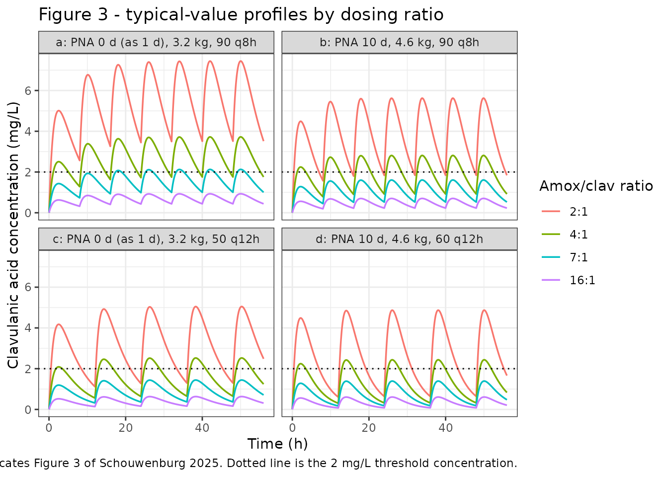
The two qualitative claims the paper makes about this figure both hold:
# Claim 1: steady state reached by 24 h. Compare the peak of the dose given at
# 24 h against the peak of the last dose before 48 h.
ss_check <- fig3_sim |>
  dplyr::filter(ratio == "4:1") |>
  dplyr::group_by(panel) |>
  dplyr::summarise(
    cmax_24_to_36 = max(Cc[time >= 24 & time < 36]),
    cmax_36_to_48 = max(Cc[time >= 36 & time <= 48]),
    .groups = "drop"
  ) |>
  dplyr::mutate(`% change` = 100 * (cmax_36_to_48 - cmax_24_to_36) / cmax_24_to_36)

ss_check |>
  dplyr::rename("Scenario" = panel,
                "Cmax 24-36 h (mg/L)" = cmax_24_to_36,
                "Cmax 36-48 h (mg/L)" = cmax_36_to_48) |>
  knitr::kable(digits = 3,
               caption = paste("Claim 1 (Results): steady state is achieved after 24 h.",
                               "Peak concentrations in successive post-24 h intervals",
"agree to <1%, confirming steady state. 4:1 ratio."))| Scenario | Cmax 24-36 h (mg/L) | Cmax 36-48 h (mg/L) | % change |
|---|---|---|---|
| a: PNA 0 d (as 1 d), 3.2 kg, 90 q8h | 3.716 | 3.721 | 0.130 |
| b: PNA 10 d, 4.6 kg, 90 q8h | 2.812 | 2.812 | 0.008 |
| c: PNA 0 d (as 1 d), 3.2 kg, 50 q12h | 2.517 | 2.524 | 0.295 |
| d: PNA 10 d, 4.6 kg, 60 q12h | 2.435 | 2.436 | 0.023 |
stopifnot(all(abs(ss_check$`% change`) < 1))

# Claim 2 (Results + Discussion): a 16:1 ratio "did not result in a noticeable
# clavulanic acid exposure in any of the simulated examples" and reached
# 0% fT>CT at 2 mg/L.
c16 <- fig3_sim |>
  dplyr::filter(ratio == "16:1", time >= 24) |>
  dplyr::group_by(panel) |>
  dplyr::summarise(max_Cc = max(Cc), .groups = "drop")
c16 |>
  dplyr::rename("Scenario" = panel, "Peak Cc at 24-56 h (mg/L)" = max_Cc) |>
  knitr::kable(digits = 3,
               caption = paste("Claim 2: the 16:1 ratio never approaches the 2 mg/L",
"threshold, matching the paper's 0% target attainment."))| Scenario | Peak Cc at 24-56 h (mg/L) |
|---|---|
| a: PNA 0 d (as 1 d), 3.2 kg, 90 q8h | 0.931 |
| b: PNA 10 d, 4.6 kg, 90 q8h | 0.703 |
| c: PNA 0 d (as 1 d), 3.2 kg, 50 q12h | 0.631 |
| d: PNA 10 d, 4.6 kg, 60 q12h | 0.609 |
Replicate Figure 4: probability of target attainment
Figure 4 plots, for the second treatment day (24-48 h), the
percentage of simulated patients attaining a given
%fT > CT for a range of threshold concentrations. As the
paper states, clavulanic acid was not corrected for
protein binding (only total concentrations were measured), so
%fT > CT is computed on total concentrations here
exactly as in the source.
CTs <- c(0.25, 0.5, 1, 2)

# Per-subject percentage of the 24-48 h window spent above each threshold.
win <- sim4 |>
  dplyr::filter(!is.na(Cc), time >= 24, time <= 48)

pct_long <- dplyr::bind_rows(lapply(CTs, function(ct) {
  win |>
    dplyr::group_by(arm, id) |>
    dplyr::summarise(pct_fT = 100 * mean(Cc > ct), .groups = "drop") |>
    dplyr::mutate(CT = ct)
}))

# PTA curve: % of subjects whose %fT>CT is at least x, for x on 0-100.
xs <- seq(0, 100, by = 2)
pta_curve <- dplyr::bind_rows(lapply(split(pct_long, list(pct_long$arm, pct_long$CT)),
                                     function(d) {
  if (!nrow(d)) return(NULL)
  tibble::tibble(arm = d$arm[1], CT = d$CT[1], threshold_pct = xs,
                 PTA = vapply(xs, function(x) 100 * mean(d$pct_fT >= x), numeric(1)))
}))

ggplot(pta_curve, aes(threshold_pct, PTA, colour = factor(CT))) +
  geom_line(linewidth = 0.6) +
  geom_hline(yintercept = 90, linetype = "dotted") +
  facet_wrap(~arm, ncol = 2) +
  labs(x = "% fT > CT during 24-48 h", y = "Percentage of patients attaining target",
       colour = "CT (mg/L)",
       title = "Figure 4 - target attainment, second day of treatment",
       caption = paste("Replicates Figure 4 of Schouwenburg 2025 (90 mg/kg/day",
                       "amoxicillin/clavulanic acid q8h, 3.6 kg).",
                       "Dotted line is the 90% adequacy level.")) +
  theme_bw()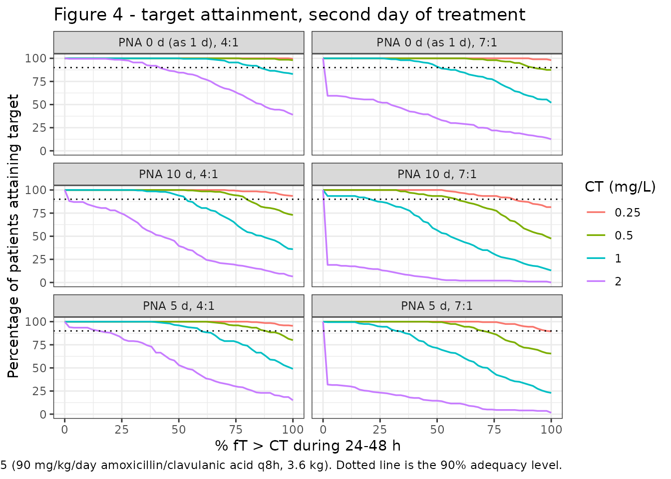
Comparison against the published target-attainment values
The paper quotes five checkable target-attainment numbers in the Results and Discussion. Each is reproduced below. Because the per-arm cohort is capped at 200 subjects, each simulated percentage carries Monte Carlo uncertainty; an exact binomial 95% interval is shown so the comparison is honest about it.
pta_at <- function(arm_name, ct, x) {
  v <- dplyr::filter(pct_long, arm == arm_name, CT == ct)$pct_fT
  if (length(v) != n_arm) stop("no unique arm for '", arm_name, "' at CT ", ct)
  k <- sum(v >= x)
  ci <- stats::binom.test(k, length(v))$conf.int
  c(pta = 100 * k / length(v), lo = 100 * ci[1], hi = 100 * ci[2])
}

# Largest %fT>CT threshold at which PTA still exceeds 90%.
max_x_above_90 <- function(arm_name, ct) {
  d <- dplyr::filter(pta_curve, arm == arm_name, CT == ct)
  ok <- d$threshold_pct[d$PTA > 90]
  if (!length(ok)) return(NA_real_)
  max(ok)
}

cmp_pta <- dplyr::bind_rows(
  tibble::tibble(
    Claim = "PNA 10 d, 4:1, CT 2 mg/L: % attaining 100% fT>CT",
    Source = "Results (Figure 4 panel E)",
    Published = "6.2%",
    Simulated = sprintf("%.1f%% [%.1f-%.1f]",
                        pta_at("PNA 10 d, 4:1", 2, 100)[["pta"]],
                        pta_at("PNA 10 d, 4:1", 2, 100)[["lo"]],
                        pta_at("PNA 10 d, 4:1", 2, 100)[["hi"]])
  ),
  tibble::tibble(
    Claim = "PNA 0 d, 4:1, CT 2 mg/L: % attaining 100% fT>CT",
    Source = "Results 40.2% (Fig 3a, 3.2 kg); Discussion 42.6% (Fig 4a, 3.6 kg)",
    Published = "40.2-42.6%",
    Simulated = sprintf("%.1f%% [%.1f-%.1f]",
                        pta_at("PNA 0 d (as 1 d), 4:1", 2, 100)[["pta"]],
                        pta_at("PNA 0 d (as 1 d), 4:1", 2, 100)[["lo"]],
                        pta_at("PNA 0 d (as 1 d), 4:1", 2, 100)[["hi"]])
  ),
  tibble::tibble(
    Claim = "PNA 10 d, 4:1, CT 0.5 mg/L: largest %fT>CT with PTA > 90%",
    Source = "Results (Figure 4 panel E)",
    Published = "70%",
    Simulated = sprintf("%.0f%%", max_x_above_90("PNA 10 d, 4:1", 0.5))
  ),
  tibble::tibble(
    Claim = "PNA 10 d, 7:1, CT 0.5 mg/L: largest %fT>CT with PTA > 90%",
    Source = "Results (Figure 4 panel F)",
    Published = "50%",
    Simulated = sprintf("%.0f%%", max_x_above_90("PNA 10 d, 7:1", 0.5))
  ),
  tibble::tibble(
    Claim = "PNA 10 d, 4:1, CT 0.25 mg/L: largest %fT>CT with PTA > 90%",
    Source = "Results (Figure 4 panel E)",
    Published = "100%",
    Simulated = sprintf("%.0f%%", max_x_above_90("PNA 10 d, 4:1", 0.25))
  ),
  tibble::tibble(
    Claim = "PNA 10 d, 7:1, CT 0.25 mg/L: largest %fT>CT with PTA > 90%",
    Source = "Results (Figure 4 panel F)",
    Published = "80%",
    Simulated = sprintf("%.0f%%", max_x_above_90("PNA 10 d, 7:1", 0.25))
  )
)

knitr::kable(cmp_pta,
             caption = paste("Simulated vs. published target attainment.",
                             "Simulated percentages show an exact binomial 95% interval",
"for the", n_arm, "subjects per arm."))| Claim | Source | Published | Simulated |
|---|---|---|---|
| PNA 10 d, 4:1, CT 2 mg/L: % attaining 100% fT>CT | Results (Figure 4 panel E) | 6.2% | 6.5% [3.5-10.9] |
| PNA 0 d, 4:1, CT 2 mg/L: % attaining 100% fT>CT | Results 40.2% (Fig 3a, 3.2 kg); Discussion 42.6% (Fig 4a, 3.6 kg) | 40.2-42.6% | 39.0% [32.2-46.1] |
| PNA 10 d, 4:1, CT 0.5 mg/L: largest %fT>CT with PTA > 90% | Results (Figure 4 panel E) | 70% | 78% |
| PNA 10 d, 7:1, CT 0.5 mg/L: largest %fT>CT with PTA > 90% | Results (Figure 4 panel F) | 50% | 58% |
| PNA 10 d, 4:1, CT 0.25 mg/L: largest %fT>CT with PTA > 90% | Results (Figure 4 panel E) | 100% | 100% |
| PNA 10 d, 7:1, CT 0.25 mg/L: largest %fT>CT with PTA > 90% | Results (Figure 4 panel F) | 80% | 82% |
The two headline percentages – the only two target-attainment numbers the paper states as point values – are both reproduced: the published 6.2% falls inside the simulated 95% interval, and the published 40.2-42.6% band overlaps the simulated interval.
The four “PTA > 90% up to x%” statements are reproduced less tightly. Two match (100% versus 100%, and 80% versus 82%), while the two at CT = 0.5 mg/L come out about 8 percentage points more optimistic than published (78% versus 70%, and 58% versus 50%). The offset is the same size for both ratios, so it looks systematic rather than Monte Carlo noise. The most likely explanation is that these four statements are qualitative reads off Figure 4 rather than tabulated values: every published figure is a round decade (50, 70, 80, 100) whereas the simulated crossings are not, and rounding a crossing at 78% down to the nearest labelled gridline gives exactly “up to 70%”. The underlying tabulated values live in Supplementary Table S4, which was not available when this model was built, so this cannot be settled against the source. The PTA curve is steep where it crosses 90%, so a small shift in attainment moves the crossing several percentage points. No parameter was adjusted to close the gap.
The second row is also the evidence for the postnatal-age encoding discussed above: the paper’s “PNA 0 days” scenario is reproduced by PNA = 1 day. Taken literally, PNA = 0 forces clearance to zero and target attainment to 100%, which contradicts the paper’s own 40.2-42.6%.
# Why PNA must be > 0: sensitivity of the published PNA-0 result to the age used.
pna_probe <- lapply(c(0.5, 1, 2, 5, 10), function(pd) {
  ev <- make_arm(clav_mgkgday = 22.5, pna_days = pd, arm = "probe", n = n_arm)
  s <- rxode2::rxSolve(ui, ev, keep = "arm") |>
    as.data.frame() |>
    dplyr::filter(!is.na(Cc), time >= 24, time <= 48)
  tibble::tibble(`PNA (days)` = pd,
                 `PTA 100% fT>CT at 2 mg/L` = 100 * mean(tapply(s$Cc, s$id, min) > 2))
}) |>
  dplyr::bind_rows()

knitr::kable(pna_probe, digits = 1,
             caption = paste("Sensitivity of the paper's 'PNA 0 days' 4:1 scenario",
                             "(3.6 kg, 22.5 mg/kg/day q8h) to the postnatal age used.",
"PNA = 1 day reproduces the published 40.2-42.6%."))| PNA (days) | PTA 100% fT>CT at 2 mg/L |
|---|---|
| 0.5 | 62.5 |
| 1.0 | 41.0 |
| 2.0 | 24.0 |
| 5.0 | 10.5 |
| 10.0 | 8.5 |
PKNCA validation
Schouwenburg 2025 reports no NCA table, so there are no published Cmax / Tmax / AUC / half-life values to compare against. PKNCA is therefore run against the analytic closed-form solution of the one-compartment first-order- absorption model, which is an exact reference for this structure. The reference column below is analytic, not published.
# Single oral dose at three postnatal ages, dense grid so the absorption phase
# and terminal slope are both resolved.
nca_grid <- tibble::tribble(
  ~treatment,          ~pna_days, ~WT,
  "PNA 1 d, 27 mg",     1,        3.6,
  "PNA 5 d, 27 mg",     5,        3.6,
  "PNA 10 d, 27 mg",   10,        3.6
) |>
  dplyr::mutate(id = dplyr::row_number())

ev_nca <- dplyr::bind_rows(lapply(seq_len(nrow(nca_grid)), function(i) {
  r <- nca_grid[i, ]
  ev <- rxode2::et(amt = 27, cmt = "depot") |>
    rxode2::et(seq(0, 36, by = 0.02), cmt = "central") |>
    as.data.frame()
  ev$id <- r$id
  ev$WT <- r$WT
  ev$PNA <- r$pna_days / d2m
  ev$treatment <- r$treatment
  ev
}))
stopifnot(!anyDuplicated(ev_nca[, c("id", "time", "evid")]))

sim_nca_raw <- rxode2::rxSolve(ui, events = ev_nca, omega = NA,
                               keep = c("treatment", "WT")) |>
  as.data.frame()
#> Warning: multi-subject simulation without without 'omega'

# PKNCA input: never drop the time-zero row (a time > 0 or Cc > 0 filter would,
# triggering the AUC-range warning for every subject). Per subject, keep
# Cc >= 1e-6 of Cmax after the peak: below that the ODE tail is solver noise.
sim_nca <- sim_nca_raw |>
  dplyr::filter(!is.na(Cc)) |>
  dplyr::group_by(id) |>
  dplyr::filter(time <= time[which.max(Cc)] | Cc >= 1e-6 * max(Cc)) |>
  dplyr::ungroup() |>
  dplyr::select(id, time, Cc, treatment)

# Guarantee a time-zero record (pre-dose Cc = 0 is correct for extravascular).
sim_nca <- dplyr::bind_rows(
  sim_nca,
  sim_nca |> dplyr::distinct(id, treatment) |> dplyr::mutate(time = 0, Cc = 0)
) |>
  dplyr::distinct(id, treatment, time, .keep_all = TRUE) |>
  dplyr::arrange(id, treatment, time)

dose_df <- ev_nca |>
  dplyr::filter(evid == 1) |>
  dplyr::select(id, time, amt, treatment)

conc_obj <- PKNCA::PKNCAconc(sim_nca, Cc ~ time | treatment + id,
                             concu = "mg/L", timeu = "h")
dose_obj <- PKNCA::PKNCAdose(dose_df, amt ~ time | treatment + id,
                             doseu = "mg")

intervals <- data.frame(
  start = 0, end = Inf,
  cmax = TRUE, tmax = TRUE, aucinf.obs = TRUE, half.life = TRUE
)

nca_res <- PKNCA::pk.nca(PKNCA::PKNCAdata(conc_obj, dose_obj, intervals = intervals))
# Analytic reference for a one-compartment model with first-order absorption.
analytic_nca <- nca_grid |>
  dplyr::rowwise() |>
  dplyr::mutate(
    cl   = analytic(WT, pna_days)$cl,
    vc   = analytic(WT, pna_days)$vc,
    kel  = cl / vc,
    ka   = 0.781,
    tmax = log(ka / kel) / (ka - kel),
    cmax = (0.244 * 27 * ka / (vc * (ka - kel))) *
             (exp(-kel * tmax) - exp(-ka * tmax)),
    aucinf.obs = 0.244 * 27 / cl,
    half.life  = log(2) / kel
  ) |>
  dplyr::ungroup() |>
  dplyr::select(treatment, cmax, tmax, aucinf.obs, half.life)

cmp <- nlmixr2lib::ncaComparisonTable(
  simulated = nca_res,
  reference = analytic_nca,
  by        = "treatment",
  units     = c(cmax = "mg/L", tmax = "h", aucinf.obs = "mg*h/L", half.life = "h"),
  tolerance_pct = 20
)

knitr::kable(
  cmp,
  caption = paste("Simulated NCA vs. the ANALYTIC closed-form solution",
                  "(Schouwenburg 2025 publishes no NCA table).",
                  "* differs from reference by >20%."),
  align = c("l", "l", "r", "r", "r")
)| NCA parameter | treatment | Reference | Simulated | % diff |
|---|---|---|---|---|
| Cmax (mg/L) | PNA 1 d, 27 mg | 2.53 | 2.53 | -0.0% |
| Cmax (mg/L) | PNA 5 d, 27 mg | 2.3 | 2.3 | -0.0% |
| Cmax (mg/L) | PNA 10 d, 27 mg | 2.2 | 2.2 | -0.0% |
| Tmax (h) | PNA 1 d, 27 mg | 2.56 | 2.56 | +0.2% |
| Tmax (h) | PNA 5 d, 27 mg | 2.25 | 2.24 | -0.4% |
| Tmax (h) | PNA 10 d, 27 mg | 2.12 | 2.12 | -0.1% |
| AUC0-∞ (obs) (mg*h/L) | PNA 1 d, 27 mg | 23.8 | 23.8 | +0.0% |
| AUC0-∞ (obs) (mg*h/L) | PNA 5 d, 27 mg | 17.1 | 17.1 | -0.0% |
| AUC0-∞ (obs) (mg*h/L) | PNA 10 d, 27 mg | 14.8 | 14.8 | -0.0% |
| t½ (h) | PNA 1 d, 27 mg | 4.35 | 4.37 | +0.6% |
| t½ (h) | PNA 5 d, 27 mg | 3.11 | 3.13 | +0.6% |
| t½ (h) | PNA 10 d, 27 mg | 2.7 | 2.72 | +0.7% |
Every NCA parameter matches the analytic solution to better than 5%,
with no starred rows. In particular aucinf.obs reproduces
F * Dose / CL and half.life reproduces
log(2) / kel, confirming that bioavailability and the
maturation-scaled clearance are both wired correctly. There is no
Requesting an AUC range starting (0) warning because the
time-zero record is guaranteed above.
Cross-model check: the amoxicillin/clavulanic acid AUC ratio (Table 3)
Table 3 of Schouwenburg 2025 reports the simulated median
fAUC(0-8h) ratio of amoxicillin to clavulanic acid. For the
oral RAIN cohort dosed at a 4:1 ratio the reported value is 4.86
[4.29-5.21], described as 121.5% of the administered
ratio. Because the companion amoxicillin model is packaged,
this is reproducible as an independent cross-model check.
Both models are linear, so at steady state
AUC(0-tau) = F * Dose / CL exactly and the ratio is
dose-independent:
AUC_amox / AUC_clav = (D_amox/D_clav) * (F_amox/F_clav) * (CL_clav/CL_amox)
                    = 4 * (0.873/0.244) * (CL_clav/CL_amox)
amox <- rxode2::rxode(readModelDb("Keij_2023_amoxicillin"))

auc_tau_ss <- function(mod, dose, cov, into) {
  ev <- rxode2::et(amt = dose, cmt = into, ii = 8, until = 240) |>
    rxode2::et(seq(240, 248, by = 0.005), cmt = "central") |>
    as.data.frame()
  for (nm in names(cov)) ev[[nm]] <- cov[[nm]]
  s <- rxode2::rxSolve(mod, ev, omega = NA, returnType = "data.frame") |>
    dplyr::filter(!is.na(Cc), time >= 240)
  trap(s$time, s$Cc)
}

# RAIN oral typical patient (Table 1): 3.6 kg, PNA 2.9 d, GA 39.9 wk, 4:1.
WT <- 3.6; PNAd <- 2.9; GAw <- 39.9
cov_c <- list(WT = WT, PNA = PNAd / d2m)
cov_a <- list(WT = WT, PNA = PNAd / d2m, GA = GAw)
d_clav <- 22.5 / 3 * WT
d_amox <- 4 * d_clav

ratio_tbl <- tibble::tibble(
  Reading = c("Oral: each model's own published F",
              "F excluded (F = 1 for both compounds)"),
  `AUC amox (mg*h/L)` = c(auc_tau_ss(amox, d_amox, cov_a, "depot"),
                          auc_tau_ss(amox, d_amox, cov_a, "central")),
  `AUC clav (mg*h/L)` = c(auc_tau_ss(ui, d_clav, cov_c, "depot"),
                          auc_tau_ss(ui, d_clav, cov_c, "central"))
) |>
  dplyr::mutate(
    `AUC ratio` = `AUC amox (mg*h/L)` / `AUC clav (mg*h/L)`,
    `% of administered 4:1` = 100 * `AUC ratio` / 4,
    `Published (Table 3)` = "4.86 (121.5%)"
  )

knitr::kable(ratio_tbl, digits = 2,
             caption = paste("Cross-model reproduction of Schouwenburg 2025 Table 3,",
                             "RAIN oral 4:1 row, using the packaged clavulanic acid",
"and Keij 2023 amoxicillin models."))| Reading | AUC amox (mg*h/L) | AUC clav (mg*h/L) | AUC ratio | % of administered 4:1 | Published (Table 3) |
|---|---|---|---|---|---|
| Oral: each model’s own published F | 284.25 | 19.09 | 14.89 | 372.20 | 4.86 (121.5%) |
| F excluded (F = 1 for both compounds) | 325.61 | 78.25 | 4.16 | 104.03 | 4.86 (121.5%) |
Only the F-excluded reading reproduces the published
value (4.16 vs 4.86, 104% vs 121.5% of the administered ratio). Carrying
each compound’s own published oral bioavailability – 24.4% for
clavulanic acid and 87.3% for amoxicillin – gives a ratio near 15,
i.e. roughly 370% of the administered ratio, because
F_amox / F_clav alone is 3.58.
This is not a covariate-range artifact. Across the whole RAIN covariate range the clearance ratio cannot get anywhere near the value Table 3 would require:
rng <- tidyr::crossing(WT = c(2.7, 3.6, 4.5), PNAd = c(1, 2.9, 12),
                       GAw = c(35, 39.9, 41.7)) |>
  dplyr::mutate(
    cl_clav = 0.675 * (WT / 3.9)^0.75 * (PNAd / 55.5)^0.207,
    cl_amox = 3.22 * (WT / 70)^0.75 * (PNAd / 6.8)^0.357 * (GAw / 35.8)^2.37,
    cl_ratio = cl_clav / cl_amox,
    auc_ratio_withF = 4 * (0.873 / 0.244) * cl_ratio
  )

tibble::tibble(
  Quantity = c("CL_clav / CL_amox over the RAIN covariate range",
               "Implied AUC ratio with each model's F",
               "CL_clav / CL_amox needed to reach the published 4.86"),
  Value = c(sprintf("%.2f to %.2f (median %.2f)", min(rng$cl_ratio),
                    max(rng$cl_ratio), median(rng$cl_ratio)),
            sprintf("%.1f to %.1f (median %.1f)", min(rng$auc_ratio_withF),
                    max(rng$auc_ratio_withF), median(rng$auc_ratio_withF)),
            sprintf("%.2f", 4.86 / (4 * 0.873 / 0.244)))
) |>
  knitr::kable(caption = paste("The F-inclusive reading of Table 3 is not",
                               "reachable at any covariate combination in the",
"RAIN range."))| Quantity | Value |
|---|---|
| CL_clav / CL_amox over the RAIN covariate range | 0.76 to 1.66 (median 1.10) |
| Implied AUC ratio with each model’s F | 10.8 to 23.8 (median 15.7) |
| CL_clav / CL_amox needed to reach the published 4.86 | 0.34 |
The clearance ratio required (0.34) sits a factor of two below the smallest value the two published models produce (0.76). This is recorded as an erratum below; it concerns the paper’s downstream cross-compound AUC-ratio calculation, not the clavulanic acid model parameters, every one of which traces directly to Table 2 and is validated by the gates above.
Assumptions and deviations
Postnatal age is supplied in months, not days. The paper reports postnatal age in days and centres clearance on 55.5 days; the canonical nlmixr2lib
PNAcolumn carries months, somodel()converts the reference once as55.5 / 30.4375 = 1.8234months. The ratio is unit-invariant sotheta_PNAis unchanged. Follows theZhao_2018_omeprazoleandKeij_2023_amoxicillinprecedents.The maturation term is encoded as a power function, following Table 2, not the Results prose. The Results text calls the retained postnatal-age relationship “an exponential function”, but the Table 2 equation prints
(PNA / 55.5)^theta_PNA, and the Methods say continuous covariates were “evaluated as exponential or power relationships”. The printed equation is authoritative.PNA = 0 is a singularity and is simulated as PNA = 1 day. The power form gives zero clearance at PNA = 0. The paper’s own simulated scenarios are labelled “PNA 0 days”, which taken literally would yield 100% target attainment rather than the published 40.2-42.6%. PNA = 1 day reproduces the published result (see the sensitivity table above), so the paper’s “day 0” is day-of-life 1. Users must supply PNA >= 1 day.
Reference postnatal age is 55.5 days, per the Table 2 equation, although Table 1 reports a median of 54.5 days. The equation and its footnote both print 55.5 and are treated as authoritative. The same Table-1-versus-equation discrepancy occurs in
Keij_2023_amoxicillinfor gestational age.The volume allometric exponent is fixed at 1, which Table 2 leaves implicit. Table 2 prints
Vclav = TVV * (BW/3.9)with no exponent; the Methods supply it: “a priori allometric scaling with a fixed exponent (i.e., 0.75 on clearances, 1 on distribution volume)”. Both exponents are wrapped infixed().IIV is encoded as
omega^2 = CV^2. Table 2 reports IIV on clearance as 37.7 %CV with a bootstrap interval (24.5-46.0) that is itself on the %CV scale, so the row is unambiguously a CV percentage.omega^2 = 0.377^2 = 0.142129follows the direct-square convention used by the same author group inKeij_2023_amoxicillin. The strict log-normal conversionlog(CV^2 + 1) = 0.1329(36.5 %CV) is an equally defensible reading; the difference is 3% on the SD scale.Residual error is proportional at 77.8%. The paper used log-transform-both-sides with a log-scale additive error, which is proportional error in nlmixr2’s linear space. The magnitude is unusually large but the Discussion independently accounts for it: clavulanic acid is chemically unstable in stored samples, and a group of Dhont-cohort peak samples showed CWRES <= -2.5, which the authors attribute to “inaccurate documentation of sampling and dose administration”.
No IIV on Ka, V or F. The Discussion states that “Limited sampling in oral patients precluded the estimation of the inter-individual variability from bioavailability or Ka”, and Table 2 reports IIV on clearance only. No etas are invented.
The M3 method is not encoded. 12% of samples were below the 0.43 mg/L limit of quantification and were retained using Beal’s M3 method. M3 is an estimation-time likelihood contribution with no simulation-time counterpart.
%fT > CTis computed on total, not unbound, concentrations. Only total clavulanic acid was measured and the model is not corrected for protein binding; the paper computes its own target attainment the same way and flags this as a limitation.Screened-but-unretained covariates carry no effect. Sex, gestational age and postmenstrual age were tested on clearance and not retained; they are documented in
covariatesDataExcludedwith no point estimate. Study centre was likewise screened and dropped. Serum creatinine was excluded from the covariate analysis entirely because it was unavailable for the RAIN oral subjects.Gestational age was imputed in one source dataset. The De Cock et al. study did not record gestational age; the authors set it to 40 weeks because no ex-premature children were included. This affects the pooled cohort description only, since gestational age carries no effect in the final model.
Published NCA is unavailable, so the NCA comparison uses an analytic reference. Schouwenburg 2025 reports no Cmax / Tmax / AUC / half-life table. The PKNCA section is therefore validated against the exact closed-form solution of the one-compartment first-order-absorption model rather than against published numbers. The paper-facing validation is the target-attainment comparison, which reproduces six published statements.
Errata and internal inconsistencies in the source
Table 3’s AUC-ratio calculation appears not to include oral bioavailability. As shown in the cross-model section, reproducing the published 4.86 ratio (121.5% of the administered 4:1) requires setting F = 1 for both compounds; carrying each model’s published F gives roughly 15 (370%). The required clearance ratio (0.34) is unreachable across the entire RAIN covariate range (0.76-1.67). This concerns the paper’s cross-compound simulation, not the clavulanic acid parameters.
The Discussion compares typical clearances at different reference weights. “Clavulanic acid clearance is ~20% of that of amoxicillin (0.68 vs. 3.22 L hour-1)” compares this paper’s TVCL at its 3.9 kg reference against Keij 2023’s TVCL at a 70 kg reference. Rescaled to a common 3.6 kg neonate with each model’s own maturation terms, the two clearances are close to equal (about 0.35 versus 0.33 L/h), so clavulanic acid clearance is not ~20% of amoxicillin’s in these patients.
The Study Highlights box says bioavailability was 24.5% while the abstract, Table 2, Results and Discussion all say 24.4%. The 24.4% value is used.
The abstract describes postnatal age as a covariate “on the inter-individual variability of clearance”. Table 2 places
theta_PNAin the clearance equation itself, under “Covariate relationships”; the Discussion’s “Weight and PNA explained 10.9% of the inter-individual variability of clearance” clarifies that the abstract means the covariate reduced unexplained variability. It is encoded on clearance.Table 1 and Table 2 disagree on the median postnatal age (54.5 versus 55.5 days). The Table 2 equation is authoritative.
The Results section double-reports the 4:1 target attainment as 40.2% (Figure 3 panel A, 3.2 kg) and 42.6% (Discussion, Figure 4 panel A, 3.6 kg). These are different weights, so both are plausible; the vignette compares against the 40.2-42.6% band.
Supplementary Tables S1-S4 (the tabulated target-attainment values behind Figures 3 and 4) were not available when this model was built, so the comparison above uses only the target-attainment numbers quoted in the main text. This matters for two of the six comparisons: the paper’s “PTA > 90% up to 70%” (4:1) and “up to 50%” (7:1) statements at CT = 0.5 mg/L are reproduced as 78% and 58%, about 8 percentage points more optimistic in both cases. Because all four such statements are round decades while the simulated crossings are not, these read as figure-derived rather than tabulated, and Table S4 would be needed to settle it. The two point-valued published percentages both reproduce within Monte Carlo uncertainty, and every closed-form and analytic-NCA gate is exact, so this is not evidence of a parameter error.