Gentamicin (Frymoyer 2013)
Source:vignettes/articles/Frymoyer_2013_gentamicin.Rmd
Frymoyer_2013_gentamicin.RmdModel and source
- Citation: Frymoyer A, Meng L, Bonifacio SL, Verotta D, Guglielmo BJ. Gentamicin pharmacokinetics and dosing in neonates with hypoxic ischemic encephalopathy receiving hypothermia. Pharmacotherapy. 2013;33(7):718-726.
- Article: https://doi.org/10.1002/phar.1263
mod_meta <- rxode2::rxode(readModelDb("Frymoyer_2013_gentamicin"))
#> ℹ parameter labels from comments will be replaced by 'label()'
mod_meta$description
#> [1] "One-compartment IV population PK model for gentamicin in 29 term neonates with hypoxic ischemic encephalopathy (HIE) receiving therapeutic hypothermia (Frymoyer 2013), with fixed allometric birth-weight scaling (exponent 0.75 on CL, 1 on Vc, reference 3.3 kg) and a power effect of serum creatinine on PNA day 1 on CL (reference 0.9 mg/dL)."
mod_meta$reference
#> [1] "Frymoyer A, Meng L, Bonifacio SL, Verotta D, Guglielmo BJ. Gentamicin pharmacokinetics and dosing in neonates with hypoxic ischemic encephalopathy receiving hypothermia. Pharmacotherapy. 2013;33(7):718-726. doi:10.1002/phar.1263."
mod_meta$units
#> $time
#> [1] "hour"
#>
#> $dosing
#> [1] "mg"
#>
#> $concentration
#> [1] "mg/L"
Population
Frymoyer 2013 developed a one-compartment population PK model from 29 term neonates with hypoxic ischemic encephalopathy (HIE) treated with whole-body therapeutic hypothermia at 33.5 degrees C in a tertiary Level III NICU (University of California San Francisco), between November 2007 and March 2010 (Table 1). Inclusion required gestational age >= 36 weeks; the cohort had median GA 40.0 weeks (IQR 37.6-40.7), median birth weight 3.32 kg (IQR 2.97-3.50), 62% female, median first arterial/capillary pH 7.0 (IQR 6.9-7.1), 10-minute APGAR median 5, 83% assisted ventilation, 55% seizures, 62% co-treated with dopamine, and 21% mortality before discharge. Serum creatinine on PNA day 1 had median 0.9 mg/dL (IQR 0.8-1.2). A total of 47 gentamicin concentrations were available for the analysis (18 patients with paired peak + trough, 11 with trough only). The standard empiric dose was 5 mg/kg every 24 h (25 neonates received that; 1 neonate received 4.5 mg/kg q24h, and 3 received 4 mg/kg q24h), administered as a 30-minute IV infusion.
Because every neonate in the cohort was undergoing therapeutic hypothermia, the paper could not evaluate hypothermia as an independent covariate; the packaged model therefore describes hypothermic-cohort PK implicitly and does not carry a hypothermia indicator (Discussion: “We were unable to evaluate the independent impact of hypothermia on gentamicin pharmacokinetics since all neonates in our study were cooled.”). For the typical study neonate (BW 3.3 kg, SCr 0.9 mg/dL), the estimated clearance of 0.034 L/h/kg was 25-50% lower than prior reports in non-asphyxiated normothermic term neonates.
The same information is available programmatically via
readModelDb("Frymoyer_2013_gentamicin")$population.
Source trace
The per-parameter origin is recorded as an in-file comment next to
each ini() entry in
inst/modeldb/specificDrugs/Frymoyer_2013_gentamicin.R. The
table below collects them in one place for review.
| Equation / parameter | Value | Source location |
|---|---|---|
lcl (log CL at reference BW 3.3 kg, SCr 0.9 mg/dL) |
log(0.111) | Frymoyer 2013 Table 2, Final Model ‘Typical Value of CL’ = 0.111 L/h (RSE 4.2%) |
lvc (log Vc at reference BW 3.3 kg) |
log(1.56) | Frymoyer 2013 Table 2, Final Model ‘V’ = 1.56 L (RSE 4.7%) |
e_wt_birth_cl (allometric BW exponent on CL) |
0.75 (fixed) | Frymoyer 2013 Methods, “Population Pharmacokinetic Analysis” |
e_wt_birth_vc (allometric BW exponent on Vc) |
1 (fixed) | Frymoyer 2013 Methods, “Population Pharmacokinetic Analysis” |
e_creat_cl (power exponent on CREAT/0.9 for CL) |
-0.566 | Frymoyer 2013 Table 2 magnitude 0.566 (RSE 21.9%); sign assigned per Results: “a typical neonate with SCr 1.4 mg/dL had a clearance 27% lower than a neonate with SCr 0.8 mg/dL” |
| IIV CL (omega^2 = log(1 + 0.161^2)) | 0.02559 (16.1% CV) | Frymoyer 2013 Table 2, Final Model ‘Inter-individual variability of CL, %CV’ (RSE 30.5%) |
propSd (proportional residual error) |
0.162 (16.2% CV) | Frymoyer 2013 Table 2, Final Model ‘Residual variability, %CV’ (RSE 24.1%) |
| Reference birth weight 3.3 kg | n/a | Frymoyer 2013 Abstract and Discussion (“the typical study neonate (BW 3.3 kg; SCr 0.9 mg/dL)”); cohort median 3.32 kg per Table 1 |
| Reference SCr 0.9 mg/dL | n/a | Frymoyer 2013 Methods: “Continuous covariates were scaled to their median values”; cohort median 0.9 mg/dL per Table 1 IQR |
| One-compartment IV PK ODE structure | n/a | Frymoyer 2013 Methods: “A one-compartment pharmacokinetic model with first-order elimination was implemented” |
| Proportional residual error | n/a | Frymoyer 2013 Results: “The residual variability … was best described by a proportional error model” |
| IIV on V removed | n/a | Frymoyer 2013 Results: “Interindividual variability for volume could not be estimated with any precision … Only interindividual variability for clearance was incorporated into the final model” |
Virtual cohort
The original observed data are not publicly available. The vignette constructs virtual cohorts that span the paper’s Table 3 dosing scenarios at the typical neonate body weight (BW 3.3 kg) and SCr (0.9 mg/dL), then verifies that simulated peak and trough concentrations match the published Table 3 values. Frymoyer 2013 used n = 5000 per arm for the published Monte Carlo simulations and inflated CL %CV to 20% (the upper end of the bootstrap CI) to bound the variability in a larger population; this vignette uses n = 200 per arm at the model’s reported 16.1% CL CV, which is sufficient to recover the published median peak / trough estimates.
The canonical covariate names in the model are WT_BIRTH
(kg) and CREAT (mg/dL).
set.seed(20260621)

n_subjects   <- 200L
infusion_h   <- 0.5         # 30-minute IV infusion (Frymoyer 2013 Methods)
n_doses      <- 6L          # enough doses to reach steady state for q48h
ref_bw_kg    <- 3.3         # typical neonate birth weight (Abstract, Discussion)
ref_scr_mgdl <- 0.9         # cohort median SCr on PNA day 1

# Frymoyer 2013 Table 3 dosing regimens (n_doses doses each so the
# last interval is steady state for all three dosing frequencies).
regimens <- tibble::tribble(
  ~regimen,          ~dose_mg_per_kg, ~interval_h,
  "5 mg/kg q24h",    5,               24,
  "5 mg/kg q36h",    5,               36,
  "5 mg/kg q48h",    5,               48,
  "4 mg/kg q24h",    4,               24,
  "4 mg/kg q36h",    4,               36
)

make_cohort <- function(n, regimen, dose_mg_per_kg, interval_h,
                        id_offset = 0L) {
  ids        <- id_offset + seq_len(n)
  amt_mg     <- ref_bw_kg * dose_mg_per_kg
  dose_times <- seq(0, by = interval_h, length.out = n_doses)
  duration_h <- max(dose_times) + interval_h

  # Observation grid: fine near each dose peak/trough plus hourly
  obs_grid <- sort(unique(c(
    seq(0, duration_h, by = 1),
    dose_times + 1.0,                                      # peak (1 h after start)
    dose_times + interval_h - 0.01,                        # trough (just before next dose)
    duration_h
  )))

  dose_rows <- tidyr::expand_grid(id = ids, time = dose_times) |>
    dplyr::mutate(
      evid     = 1L,
      cmt      = "central",
      amt      = amt_mg,
      rate     = amt_mg / infusion_h,
      WT_BIRTH = ref_bw_kg,
      CREAT    = ref_scr_mgdl,
      regimen  = regimen
    )

  obs_rows <- tidyr::expand_grid(id = ids, time = obs_grid) |>
    dplyr::mutate(
      evid     = 0L,
      cmt      = "central",
      amt      = 0,
      rate     = 0,
      WT_BIRTH = ref_bw_kg,
      CREAT    = ref_scr_mgdl,
      regimen  = regimen
    )

  dplyr::bind_rows(dose_rows, obs_rows) |>
    dplyr::arrange(id, time, dplyr::desc(evid))
}

events <- dplyr::bind_rows(
  lapply(seq_len(nrow(regimens)), function(k) {
    make_cohort(
      n               = n_subjects,
      regimen         = regimens$regimen[k],
      dose_mg_per_kg  = regimens$dose_mg_per_kg[k],
      interval_h      = regimens$interval_h[k],
      id_offset       = (k - 1L) * 1000L
    )
  })
)

stopifnot(!anyDuplicated(unique(events[, c("id", "time", "evid")])))

cat(
  "Cohorts:", nrow(regimens),
  " | Dose rows:", sum(events$evid == 1L),
  " | Obs rows:", sum(events$evid == 0L), "\n"
)
#> Cohorts: 5  | Dose rows: 6000  | Obs rows: 208600
Simulation
mod <- readModelDb("Frymoyer_2013_gentamicin")
sim <- rxode2::rxSolve(
  mod,
  events = events,
  keep   = c("regimen", "WT_BIRTH", "CREAT")
) |>
  as.data.frame()
#> ℹ parameter labels from comments will be replaced by 'label()'
Replicate published figures
Figure 2 – typical concentration-time profile (5 mg/kg q24h, q36h, q48h)
Frymoyer 2013 Figure 2 (visual predictive check) shows simulated gentamicin concentrations dose-normalised to 5 mg/kg. The panel below plots the median and 5th-95th percentile concentration-time curves over the dosing window for the three steady-state intervals at 5 mg/kg.
ribbon_df <- sim |>
  dplyr::filter(!is.na(Cc), regimen %in% c("5 mg/kg q24h",
                                           "5 mg/kg q36h",
                                           "5 mg/kg q48h")) |>
  dplyr::group_by(regimen, time) |>
  dplyr::summarise(
    Q05 = quantile(Cc, 0.05, na.rm = TRUE),
    Q50 = quantile(Cc, 0.50, na.rm = TRUE),
    Q95 = quantile(Cc, 0.95, na.rm = TRUE),
    .groups = "drop"
  )

ggplot(ribbon_df, aes(time, Q50)) +
  geom_hline(yintercept = 6, linetype = "dashed", colour = "steelblue") +
  geom_hline(yintercept = 2, linetype = "dashed", colour = "firebrick") +
  geom_ribbon(aes(ymin = Q05, ymax = Q95), alpha = 0.30) +
  geom_line() +
  facet_wrap(~ regimen, ncol = 1, scales = "free_x") +
  scale_x_continuous(breaks = seq(0, 14 * 24, 24)) +
  labs(
    x       = "Time after first dose (h)",
    y       = "Gentamicin Cc (mg/L)",
    title   = "Concentration-time profile at 5 mg/kg by dosing interval",
    caption = paste0(
      "Median (solid) and 5th-95th percentile (shaded) across ",
      n_subjects, " virtual subjects at BW 3.3 kg, SCr 0.9 mg/dL. ",
      "Blue dashed = 6 mg/L peak target; red dashed = 2 mg/L trough ceiling."
    )
  )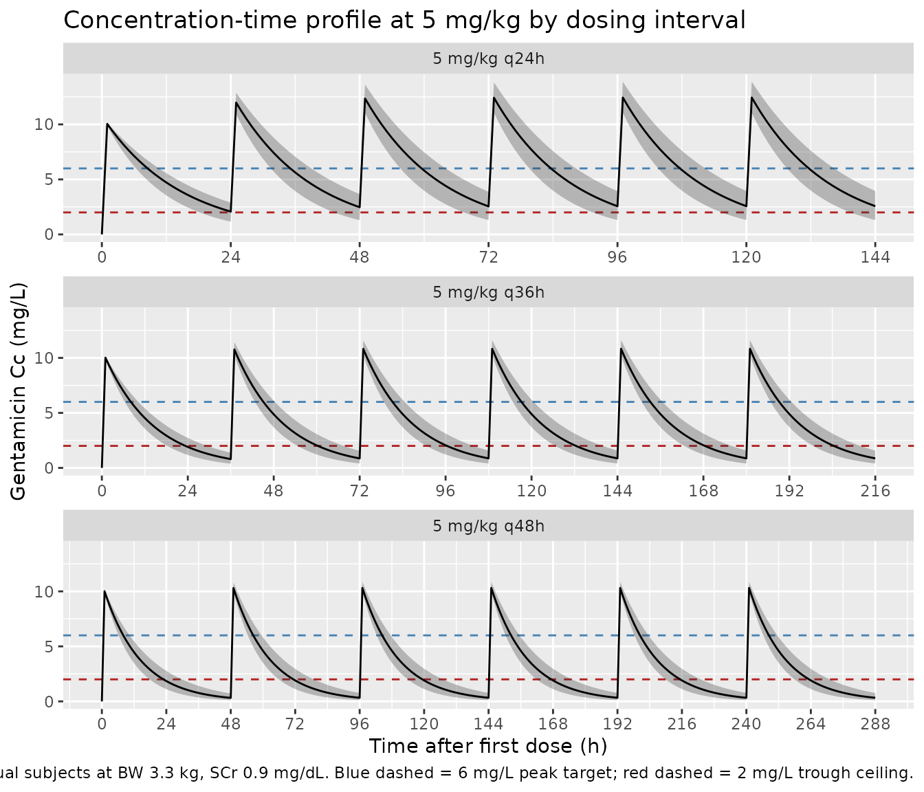
Figure 3 – target attainment by dose and interval
Frymoyer 2013 Figure 3 reports the fraction of neonates achieving (a) steady-state trough < 2 mg/L, (b) post-first-dose peak > 6 mg/L, and (c) steady-state peak > 6 mg/L, at doses 3-5 mg/kg with intervals of 24, 36, or 48 h. The chunk below recomputes the steady-state trough attainment (panel a) across the five regimens simulated above.
# Steady-state interval = last interval of the simulation window.
ss_intervals <- regimens |>
  dplyr::mutate(
    ss_start = (n_doses - 1) * interval_h,
    ss_end   = n_doses * interval_h
  )

ss_troughs <- sim |>
  dplyr::filter(!is.na(Cc)) |>
  dplyr::inner_join(ss_intervals, by = "regimen") |>
  dplyr::group_by(id, regimen) |>
  dplyr::filter(time >= ss_start, time <= ss_end) |>
  dplyr::slice_max(time, n = 1, with_ties = FALSE) |>
  dplyr::ungroup() |>
  dplyr::select(id, regimen, trough = Cc)

target_attainment <- ss_troughs |>
  dplyr::group_by(regimen) |>
  dplyr::summarise(
    pct_trough_lt_2 = mean(trough < 2) * 100,
    .groups = "drop"
  )

knitr::kable(
  target_attainment,
  digits = 1,
  col.names = c("Regimen", "% with steady-state trough < 2 mg/L"),
  caption  = paste(
    "Steady-state trough attainment by regimen. Compare with",
    "Frymoyer 2013 Figure 3a (24-hour dosing fails to reliably",
    "achieve trough < 2 mg/L; 36-hour and 48-hour dosing both",
    "exceed 90% target attainment)."
  )
)| Regimen | % with steady-state trough < 2 mg/L |
|---|---|
| 4 mg/kg q24h | 59 |
| 4 mg/kg q36h | 100 |
| 5 mg/kg q24h | 28 |
| 5 mg/kg q36h | 99 |
| 5 mg/kg q48h | 100 |
PKNCA validation
Compute Cmax (peak) and Cmin (trough) per subject over the last
steady-state dosing interval using PKNCA, grouped by
regimen. Frymoyer 2013 defines peak as the concentration 30
minutes after the end of a 30-minute infusion (i.e. 1 hour after dose
start) and trough as the concentration just before the next dose.
sim_nca <- sim |>
  dplyr::filter(!is.na(Cc)) |>
  dplyr::inner_join(ss_intervals, by = "regimen") |>
  dplyr::filter(time >= ss_start, time <= ss_end) |>
  dplyr::mutate(time_in_interval = time - ss_start) |>
  dplyr::ungroup() |>
  dplyr::select(id, time_in_interval, Cc, regimen)

# Guarantee a time=0 row per (id, regimen) for PKNCA's AUC anchor.
# At steady state, the start-of-interval concentration equals the
# concentration carried over from the previous trough; PKNCA will use
# the supplied value to anchor AUC. We bind in the start-of-interval
# concentration that the simulation produced at ss_start.
ss_anchor <- sim |>
  dplyr::filter(!is.na(Cc)) |>
  dplyr::inner_join(ss_intervals, by = "regimen") |>
  dplyr::filter(abs(time - ss_start) < 1e-6) |>
  dplyr::transmute(id, regimen, time_in_interval = 0, Cc)

sim_nca <- dplyr::bind_rows(sim_nca, ss_anchor) |>
  dplyr::distinct(id, regimen, time_in_interval, .keep_all = TRUE) |>
  dplyr::arrange(id, regimen, time_in_interval)

conc_obj <- PKNCA::PKNCAconc(
  sim_nca, Cc ~ time_in_interval | regimen + id,
  concu = "mg/L", timeu = "h"
)

# Dose at t = 0 of the steady-state interval; per-cohort amount.
dose_amt <- regimens$dose_mg_per_kg * ref_bw_kg
names(dose_amt) <- regimens$regimen

dose_df <- sim_nca |>
  dplyr::distinct(id, regimen) |>
  dplyr::mutate(
    time_in_interval = 0,
    amt              = dose_amt[as.character(regimen)]
  )

dose_obj <- PKNCA::PKNCAdose(
  dose_df, amt ~ time_in_interval | regimen + id,
  doseu = "mg"
)

intervals <- data.frame(
  start    = 0,
  end      = max(regimens$interval_h),
  cmax     = TRUE,
  cmin     = TRUE,
  tmax     = TRUE,
  auclast  = TRUE
)

nca_data <- PKNCA::PKNCAdata(conc_obj, dose_obj, intervals = intervals)
nca_res  <- PKNCA::pk.nca(nca_data)
Comparison against Frymoyer 2013 Table 3
Frymoyer 2013 Table 3 reports simulated steady-state peak and trough concentrations as median (10%, 90%) for each regimen (5,000 subjects per arm with CL %CV inflated to 20% and BW / SCr distributions from the CDC and the cohort, respectively). The chunk below recomputes the same statistics from the packaged-model simulation at the typical neonate (BW 3.3 kg, SCr 0.9 mg/dL) and renders them side-by-side with the published values.
peak_h <- 1.0   # 30 min after end of 30 min infusion

peaks <- sim |>
  dplyr::filter(!is.na(Cc)) |>
  dplyr::inner_join(ss_intervals, by = "regimen") |>
  dplyr::filter(abs(time - (ss_start + peak_h)) < 1e-6) |>
  dplyr::select(id, regimen, peak = Cc)

troughs <- ss_troughs

simulated_summary <- dplyr::left_join(peaks, troughs,
                                      by = c("id", "regimen")) |>
  dplyr::group_by(regimen) |>
  dplyr::summarise(
    median_trough_sim = median(trough, na.rm = TRUE),
    median_peak_sim   = median(peak,   na.rm = TRUE),
    p10p90_trough_sim = paste0(
      sprintf("%.1f-%.1f",
              quantile(trough, 0.10, na.rm = TRUE),
              quantile(trough, 0.90, na.rm = TRUE))
    ),
    p10p90_peak_sim   = paste0(
      sprintf("%.1f-%.1f",
              quantile(peak, 0.10, na.rm = TRUE),
              quantile(peak, 0.90, na.rm = TRUE))
    ),
    .groups = "drop"
  )

published <- tibble::tribble(
  ~regimen,          ~median_trough_pub, ~p10p90_trough_pub, ~median_peak_pub, ~p10p90_peak_pub,
  "5 mg/kg q24h",    2.3,                "1.0-4.5",          11.8,             "8.5-15.7",
  "5 mg/kg q36h",    0.9,                "0.3-2.0",          10.5,             "7.8-13.5",
  "5 mg/kg q48h",    0.4,                "0.1-1.0",          10.0,             "7.3-12.8",
  "4 mg/kg q24h",    1.8,                "0.8-3.6",          9.4,              "6.8-12.5",
  "4 mg/kg q36h",    0.7,                "0.2-1.6",          8.4,              "6.2-10.8"
)

comparison <- published |>
  dplyr::left_join(simulated_summary, by = "regimen") |>
  dplyr::select(regimen,
                median_trough_pub, median_trough_sim,
                p10p90_trough_pub, p10p90_trough_sim,
                median_peak_pub,   median_peak_sim,
                p10p90_peak_pub,   p10p90_peak_sim)

knitr::kable(
  comparison,
  digits  = 2,
  caption = paste(
    "Simulated vs Frymoyer 2013 Table 3 (steady-state median trough",
    "and peak with 10%-90% interval, mg/L). The 'pub' columns are the",
    "published Monte Carlo values (n = 5000, CL CV inflated to 20%);",
    "the 'sim' columns are recomputed from the packaged model",
    "(n = ", n_subjects, ", CL CV 16.1% as reported in Table 2),",
    "at the typical neonate BW 3.3 kg / SCr 0.9 mg/dL. Medians should",
    "track closely; the simulated 10%-90% range is tighter because",
    "the packaged model uses the as-fit IIV rather than the inflated",
    "variability and holds BW and SCr at their reference values."
  )
)| regimen | median_trough_pub | median_trough_sim | p10p90_trough_pub | p10p90_trough_sim | median_peak_pub | median_peak_sim | p10p90_peak_pub | p10p90_peak_sim |
|---|---|---|---|---|---|---|---|---|
| 5 mg/kg q24h | 2.3 | 2.57 | 1.0-4.5 | 1.5-3.7 | 11.8 | 12.44 | 8.5-15.7 | 11.2-13.6 |
| 5 mg/kg q36h | 0.9 | 0.87 | 0.3-2.0 | 0.5-1.4 | 10.5 | 10.83 | 7.8-13.5 | 10.4-11.5 |
| 5 mg/kg q48h | 0.4 | 0.33 | 0.1-1.0 | 0.1-0.7 | 10.0 | 10.31 | 7.3-12.8 | 10.0-10.8 |
| 4 mg/kg q24h | 1.8 | 1.88 | 0.8-3.6 | 1.2-2.8 | 9.4 | 9.77 | 6.8-12.5 | 9.0-10.8 |
| 4 mg/kg q36h | 0.7 | 0.65 | 0.2-1.6 | 0.4-1.1 | 8.4 | 8.61 | 6.2-10.8 | 8.3-9.2 |
res_tbl <- as.data.frame(nca_res$result)
knitr::kable(
  utils::head(res_tbl[, c("start", "end", "regimen", "PPTESTCD", "PPORRES")], 20),
  caption = "First 20 rows of per-subject PKNCA output (long form).",
  digits  = 3,
  row.names = FALSE
)| start | end | regimen | PPTESTCD | PPORRES |
|---|---|---|---|---|
| 0 | 48 | 4 mg/kg q24h | auclast | 103.598 |
| 0 | 48 | 4 mg/kg q24h | cmax | 9.338 |
| 0 | 48 | 4 mg/kg q24h | cmin | 1.483 |
| 0 | 48 | 4 mg/kg q24h | tmax | 1.000 |
| 0 | 48 | 4 mg/kg q24h | auclast | 131.958 |
| 0 | 48 | 4 mg/kg q24h | cmax | 10.346 |
| 0 | 48 | 4 mg/kg q24h | cmin | 2.424 |
| 0 | 48 | 4 mg/kg q24h | tmax | 1.000 |
| 0 | 48 | 4 mg/kg q24h | auclast | 139.619 |
| 0 | 48 | 4 mg/kg q24h | cmax | 10.628 |
| 0 | 48 | 4 mg/kg q24h | cmin | 2.692 |
| 0 | 48 | 4 mg/kg q24h | tmax | 1.000 |
| 0 | 48 | 4 mg/kg q24h | auclast | 136.544 |
| 0 | 48 | 4 mg/kg q24h | cmax | 10.515 |
| 0 | 48 | 4 mg/kg q24h | cmin | 2.584 |
| 0 | 48 | 4 mg/kg q24h | tmax | 1.000 |
| 0 | 48 | 4 mg/kg q24h | auclast | 124.338 |
| 0 | 48 | 4 mg/kg q24h | cmax | 10.070 |
| 0 | 48 | 4 mg/kg q24h | cmin | 2.162 |
| 0 | 48 | 4 mg/kg q24h | tmax | 1.000 |
Assumptions and deviations
- Reference birth weight 3.3 kg. The Abstract and Discussion use 3.3 kg as the typical neonate weight to which the published clearance estimate 0.034 L/h/kg corresponds (giving CL = 0.111 L/h at 3.3 kg, matching Table 2). The cohort median birth weight in Table 1 is 3.32 kg; the difference between 3.3 and 3.32 changes CL by 0.5% and is immaterial for replication of Table 3.
- Reference SCr 0.9 mg/dL. The cohort median SCr on PNA day 1 is 0.9 mg/dL (Table 1 IQR 0.8-1.2). Methods state “Continuous covariates were scaled to their median values”; 0.9 mg/dL is the median used.
-
Sign of the SCr exponent. Table 2 prints the
exponent magnitude (0.566) but the equation form is not written out as a
decoded formula in the manuscript. The Results narrative provides the
direction: “a typical neonate with SCr 1.4 mg/dL had a clearance 27%
lower than a neonate with SCr 0.8 mg/dL”. Setting
e_creat_cl = -0.566and computing(1.4/0.8)^(-0.566) = 0.729reproduces the published 27.1% reduction; the positive form(1.4/0.8)^(+0.566) = 1.37would imply 37% higher CL at higher SCr, contradicting the narrative. The packaged model encodes the negative sign explicitly with a comment. - Hypothermia not modelled as a covariate. Every neonate in the cohort was undergoing whole-body hypothermia at 33.5 degrees C. Discussion: “We were unable to evaluate the independent impact of hypothermia on gentamicin pharmacokinetics since all neonates in our study were cooled.” The model therefore characterises hypothermic- cohort PK implicitly; the population metadata records the disease state, and users intending to apply this model to normothermic neonates should consult alternatives such as Bijleveld 2017 or Fuchs 2014 which include broader gestational-age and ventilation strata.
- IIV magnitude in the packaged model differs from Frymoyer 2013 Table 3 simulations. The packaged model uses the as-reported IIV CL = 16.1% CV (Table 2). For the Table 3 Monte Carlo simulations the paper inflated CL %CV to 20% (the upper bound of the bootstrap 95% CI) to mimic increased variability expected in a larger population. The vignette’s simulated 10-90% percentile ranges are therefore narrower than the published Table 3 ranges; the medians should track closely because they are driven by the typical-value structural predictions at the reference BW / SCr.
-
GA, PNA, first arterial pH, 10-minute APGAR, and dopamine
were not retained. The paper screened these covariates during
forward selection and found none significantly affected gentamicin
clearance (Results “Population Pharmacokinetic Analysis”). The packaged
model retains only BW (allometric) and SCr (power) on CL. The screened-
but-not-retained covariates are documented in
covariatesDataExcludedfor provenance. - IIV on V was removed from the final model. Results: “Interindividual variability for volume could not be estimated with any precision using the available data … it was removed from the model.” The packaged model carries IIV on CL only.
-
Infusion duration set by the event table. The model
does not hard-code
dur(central). Users specify infusion duration per dose via therate(ordur) column on event-table dose rows; the vignette usesrate = amt / 0.5to deliver each 30-minute infusion as in the source paper. - Errata not located. A targeted search of the journal landing page and Google Scholar at extraction time did not turn up an erratum for this article. If one is later identified that revises a Table 2 estimate, the packaged values should be refreshed accordingly.