Epoetin alfa (Perez-Ruixo 2008)
Source:vignettes/articles/PerezRuixo_2008_epoetinAlfa.Rmd
PerezRuixo_2008_epoetinAlfa.RmdModel and source
- Citation: Perez-Ruixo JJ, Krzyzanski W, Hing J. Pharmacodynamic analysis of recombinant human erythropoietin effect on reticulocyte production rate and age distribution in healthy subjects. Clin Pharmacokinet. 2008;47(6):399-415. doi:10.2165/00003088-200847060-00004. PK structure and prior typical values + prior CV% adopted from Olsson-Gisleskog P, Jacqmin P, Perez-Ruixo JJ. Population pharmacokinetics meta-analysis of recombinant human erythropoietin in healthy subjects. Clin Pharmacokinet. 2007;46(2):159-73. doi:10.2165/00003088-200746020-00004 (MAP-Bayesian POSTHOC PK inputs to the PD analysis; see Table I).
- Description: Population PK/PD model for subcutaneous recombinant human erythropoietin (rHuEPO / epoetin alfa) in healthy adult male volunteers (Perez-Ruixo 2008). PK is the Olsson-Gisleskog 2007 prior (two-compartment with linear + Michaelis-Menten elimination and dual subcutaneous absorption: a fast sequential zero-order infusion into the depot of duration D1 feeding first-order absorption ka into central, plus a slower zero-order direct infusion into central of duration D2 after lag time tlag2; dose-dependent absolute bioavailability F = F0 + Emax(F)Dose/(ED50(F)+Dose)). Endogenous EPO is maintained at the baseline BSL by a constant input rate kEPO derived from the steady-state balance against linear + MM elimination (equation 4). The PD layer is the maturation-structured cytokinetic model D: rHuEPO stimulates the progenitor production rate kinC/(SC50+C) into a 10-stage bone-marrow precursor age chain (transfer rate Np/Tp), which feeds a 10-stage circulating reticulocyte age chain whose transfer rate (NR/TR)*(S0/SM) is inhibited by a 5-stage signal transduction (transit time tau) driven by C/(EC50+C). Output RET = sum of reticulocyte compartments reproduces the percentage of reticulocytes in % units. No demographic covariate effects were retained in either layer.
- Article: https://doi.org/10.2165/00003088-200847060-00004
- Upstream popPK source for the PK structure and PK priors: Olsson-Gisleskog et al. (2007) Clin Pharmacokinet 46(2):159-173, https://doi.org/10.2165/00003088-200746020-00004.
Population
Perez-Ruixo et al. (2008) pooled 88 healthy adult male volunteers from three open-label, randomized, placebo-controlled, parallel-group phase I studies (study A 1996 n=20; study B 1996 n=20; study C 2002 n=48; one study-C subject discontinued and was excluded from the PD analysis). Subjects were 18-45 years of age and 63.6-100 kg. Inclusion required baseline serum erythropoietin < 30 IU/L, haemoglobin 13.8-16.4 g/dL, haematocrit 41-49%, baseline reticulocytes <= 3%, normal serum folate, vitamin B12 and iron, and daily oral iron supplementation (equivalent to 210 mg elemental iron) through day 29 of the study. A single subcutaneous rHuEPO dose was administered; absolute doses spanned 20-160 kIU (per-kg doses in studies A and B were converted to absolute IU for analysis). 2018 rHuEPO serum concentrations and 1628 reticulocyte percentages entered the PK and PD analyses respectively.
The population metadata is available programmatically:
str(.mod_ui$population, max.level = 1)
#> List of 13
#>  $ species          : chr "human"
#>  $ n_subjects       : int 88
#>  $ n_studies        : int 3
#>  $ age_range        : chr "18-45 years"
#>  $ weight_range     : chr "63.6-100 kg"
#>  $ sex_female_pct   : num 0
#>  $ race_ethnicity   : chr "Not separately tabulated in Perez-Ruixo 2008."
#>  $ disease_state    : chr "Healthy adult male volunteers; physical exam, ECG and standard laboratory tests confirmed healthy. Baseline ser"| __truncated__
#>  $ dose_range       : chr "Single subcutaneous rHuEPO dose. Study A (1996, n=20): 300/600/1200/2400 IU/kg. Study B (1996, n=20): 450/900/1"| __truncated__
#>  $ regions          : chr "Study A and B: South Florida Bioavailability Clinic (Miami, FL, USA). Study C: Chiltern International (Buckinghamshire, UK)."
#>  $ n_pk_observations: int 2018
#>  $ n_pd_observations: int 1628
#>  $ notes            : chr "Three open-label, randomized, placebo-controlled, parallel-group phase I studies pooled. Serum rHuEPO by modifi"| __truncated__
Source trace
The PK structure (equations 1-5 and Table I including the footnote-a
fixed values) comes from Olsson-Gisleskog 2007 and is used as the prior
for the MAP-Bayesian POSTHOC individual PK estimation in this paper. The
PD structure (equations 6-13 and 21-25 for Model D; equations 26-27 for
the random-effects model) is the novel contribution of Perez-Ruixo 2008.
The table below collects the per-parameter provenance; the in-file
inst/modeldb/specificDrugs/PerezRuixo_2008_epoetinAlfa.R
comments record the same.
| Symbol | File parameter | Value | Source location |
|---|---|---|---|
| ka | lka | 0.034 1/h | Perez-Ruixo 2008 Table I, Prior mean (Olsson-Gisleskog 2007) |
| CLI | lcl | 0.358 L/h | Perez-Ruixo 2008 Table I, Prior mean |
| V2 | lvc | 3.89 L | Perez-Ruixo 2008 Table I, Prior mean |
| Vmax | lvmax | 211 IU/h | Perez-Ruixo 2008 Table I, Prior mean |
| D1 | ld1 | 0.725 h | Perez-Ruixo 2008 Table I, Prior mean |
| tlag2 | ltlag2 | 2.72 h | Perez-Ruixo 2008 Table I, Prior mean |
| F0 | lfdepot | 0.62 | Perez-Ruixo 2008 Table I, Prior mean |
| BSL | lrbase | 13.9 IU/L | Perez-Ruixo 2008 Table I, Prior mean |
| fr | logitfr | 0.60 (logit) | Perez-Ruixo 2008 Table I, Prior mean |
| Km | lkm | 394 IU/L (fixed) | Perez-Ruixo 2008 Table I footnote a |
| Q | lq | 0.044 L/h (fixed) | Perez-Ruixo 2008 Table I footnote a |
| V3 | lvp | 1.64 L (fixed) | Perez-Ruixo 2008 Table I footnote a |
| D2 | ld2 | 37.8 h (fixed) | Perez-Ruixo 2008 Table I footnote a |
| Emax(F) | lemax_f | 0.649 (fixed) | Perez-Ruixo 2008 Table I footnote a |
| ED50(F) | led50_f | 63200 IU (fixed) | Perez-Ruixo 2008 Table I footnote a |
| RET0 | lret0 | 1.24 % | Perez-Ruixo 2008 Table II Model D, Original dataset |
| TR | ltr | 62.2 h | Perez-Ruixo 2008 Table II Model D, Original dataset |
| Tp | ltp | 118 h | Perez-Ruixo 2008 Table II Model D, Original dataset |
| SC50 | lsc50 | 7.61 IU/L | Perez-Ruixo 2008 Table II Model D, Original dataset |
| EC50 | lec50 | 56.3 IU/L | Perez-Ruixo 2008 Table II Model D, Original dataset |
| tau | ltau | 4.89 h | Perez-Ruixo 2008 Table II Model D, Original dataset |
| sigma | propSd_RET | 0.631 (CV) | Perez-Ruixo 2008 Table II Model D, Original dataset |
| Eq. 1-3 | PK ODEs | n/a | Perez-Ruixo 2008 Methods, “Pharmacokinetic Analysis” |
| Eq. 4 | kEPO | n/a | Perez-Ruixo 2008 Methods (endogenous EPO steady-state) |
| Eq. 5 | f_total | n/a | Perez-Ruixo 2008 Methods (dose-dependent F) |
| Eq. 6-13 | Model A + ICs | n/a | Perez-Ruixo 2008 Methods, “Model A” |
| Eq. 21-25 | Model D signal | n/a | Perez-Ruixo 2008 Methods, “Model D” |
Units check
The model is wired in hours (time), IU (mass dose), and IU/L
(concentration); the PD output RET is in absolute
percentage units (e.g., 1.24 = 1.24 %). Walking the ODE for the first
precursor compartment:
units of kin         = % / h           (= RET0 / TR = 1.24 % / 62.2 h)
units of C/(SC50+C)  = dimensionless
units of P_1         = % (carries through the catenary chain)
units of k_p * P_1   = (1/h) * %       = % / h
=> d/dt(P_1)         = % / h           consistent with d/dt(state) on the LHS
The signal-transduction chain is dimensionless (each
transit_k(0) = sig0 is dimensionless),
aging_mod = sig0 / transit5 is dimensionless, and the
reticulocyte ODE d/dt(retic_j) = k_r * aging_mod * (...)
carries % / h consistently. The PK ODE d/dt(central)
carries IU / h: each ka * depot, kEPO, CLI * Cc, MM term, and Q-flux is
IU / h.
Loading the model
mod  <- .mod_ui                # already loaded in the hidden `meta` chunk above
mtyp <- rxode2::zeroRe(mod)    # typical-value (no IIV); reproduces Fig 4 medians
Validation 1 – pre-dose endogenous steady state
With central(0) = BSL * vc,
peripheral1(0) = BSL * V3, the constant endogenous
production kEPO = CLI*BSL + Vmax*BSL/(Km+BSL) exactly
balances linear + MM elimination at the baseline endogenous
concentration. The precursor and reticulocyte chains start at their
RET0-driven steady state (equations 11 and 13), and the
signal-transduction transit chain starts at
sig0 = BSL/(EC50+BSL). The system should hold its baseline
indefinitely in the absence of any exogenous dose.
ev_baseline <- tibble::tibble(
  id   = 1L,
  time = seq(0, 24*7, by = 6),
  amt  = 0,
  rate = 0,
  evid = 0L,
  cmt  = NA_character_,
  dvid = 1L,
  DOSE = 0
)
s_baseline <- rxode2::rxSolve(mtyp, ev_baseline) |>
  as.data.frame()
#> ℹ omega/sigma items treated as zero: 'etalka', 'etalcl', 'etalvc', 'etalvmax', 'etald1', 'etaltlag2', 'etalfdepot', 'etalrbase', 'etalogitfr', 'etalret0', 'etaltr', 'etaltp', 'etalsc50'
range(s_baseline$Cc)
#> [1] 13.9 13.9
range(s_baseline$RET)
#> [1] 1.24 1.24
Cc should stay at 13.9 IU/L and RET should
stay at 1.24 % across the seven-day no-dose simulation.
Validation 2 – replicate Figure 4 (PK + PD median trajectories)
Perez-Ruixo 2008 Figure 4 shows the time courses of rHuEPO serum concentration (panel a) and reticulocyte percentage (panel b) for the six study-C doses (20, 40, 60, 90, 120, 160 kIU). Lines and shaded areas in the paper are the median and 90% prediction interval from the posterior predictive check. The typical-value (no-IIV) simulation here reproduces the median.
The dose-record convention: rxode2’s solver does not accept two
simultaneous rate=-2 records (one to depot, one to
central); the central dose record is therefore timed at
time = 1e-3 h so it is distinct from the depot record at
time = 0. The model’s alag(central) = tlag2
then shifts the actual central-compartment administration to
1e-3 + tlag2 ~ tlag2 – the slow pathway’s intended ~ 2.72 h
lag from Olsson-Gisleskog 2007.
make_events <- function(dose_kIU, obs_times) {
  dose_amt <- dose_kIU * 1000  # IU
  doses <- dplyr::bind_rows(
    tibble::tibble(time = 0,    amt = dose_amt, rate = -2, evid = 1L,
                   cmt = "depot",   dvid = NA_integer_),
    tibble::tibble(time = 1e-3, amt = dose_amt, rate = -2, evid = 1L,
                   cmt = "central", dvid = NA_integer_)
  )
  obs <- dplyr::bind_rows(
    tibble::tibble(time = obs_times, amt = 0, rate = 0, evid = 0L,
                   cmt = NA_character_, dvid = 1L),
    tibble::tibble(time = obs_times, amt = 0, rate = 0, evid = 0L,
                   cmt = NA_character_, dvid = 2L)
  )
  dplyr::bind_rows(doses, obs) |>
    dplyr::mutate(id = 1L,
                  DOSE = dose_amt,
                  treatment = paste0(dose_kIU, " kIU")) |>
    dplyr::arrange(time, dplyr::desc(evid))
}

dose_levels <- c(20, 40, 60, 90, 120, 160)
obs_pk_h  <- unique(c(seq(0, 24, by = 1), seq(24, 24*15, by = 6)))
obs_pd_h  <- unique(c(seq(0, 24*15, by = 6), seq(24*15, 24*45, by = 12)))
obs_times <- sort(unique(c(obs_pk_h, obs_pd_h)))

events <- dplyr::bind_rows(lapply(dose_levels, make_events, obs_times = obs_times))
events$id <- match(events$treatment, paste0(dose_levels, " kIU"))
sim <- rxode2::rxSolve(
  mtyp,
  events,
  keep        = c("treatment", "DOSE")
) |> as.data.frame()
#> ℹ omega/sigma items treated as zero: 'etalka', 'etalcl', 'etalvc', 'etalvmax', 'etald1', 'etaltlag2', 'etalfdepot', 'etalrbase', 'etalogitfr', 'etalret0', 'etaltr', 'etaltp', 'etalsc50'
#> Warning: multi-subject simulation without without 'omega'
nrow(sim)
#> [1] 1692
sim |>
  dplyr::filter(time <= 24*15) |>
  dplyr::mutate(treatment = factor(treatment, levels = paste0(dose_levels, " kIU"))) |>
  ggplot2::ggplot(ggplot2::aes(time, Cc, group = treatment)) +
  ggplot2::geom_line(color = "steelblue", size = 0.6) +
  ggplot2::geom_hline(yintercept = 13.9, linetype = "dashed", color = "grey50") +
  ggplot2::facet_wrap(~ treatment, ncol = 3) +
  ggplot2::scale_y_log10(limits = c(5, 5000)) +
  ggplot2::labs(x = "Time (h)", y = "rHuEPO serum concentration (IU/L)",
                title = "Figure 4(a) -- typical-value PK profile") +
  ggplot2::theme_minimal()
#> Warning: Using `size` aesthetic for lines was deprecated in ggplot2 3.4.0.
#> ℹ Please use `linewidth` instead.
#> This warning is displayed once per session.
#> Call `lifecycle::last_lifecycle_warnings()` to see where this warning was
#> generated.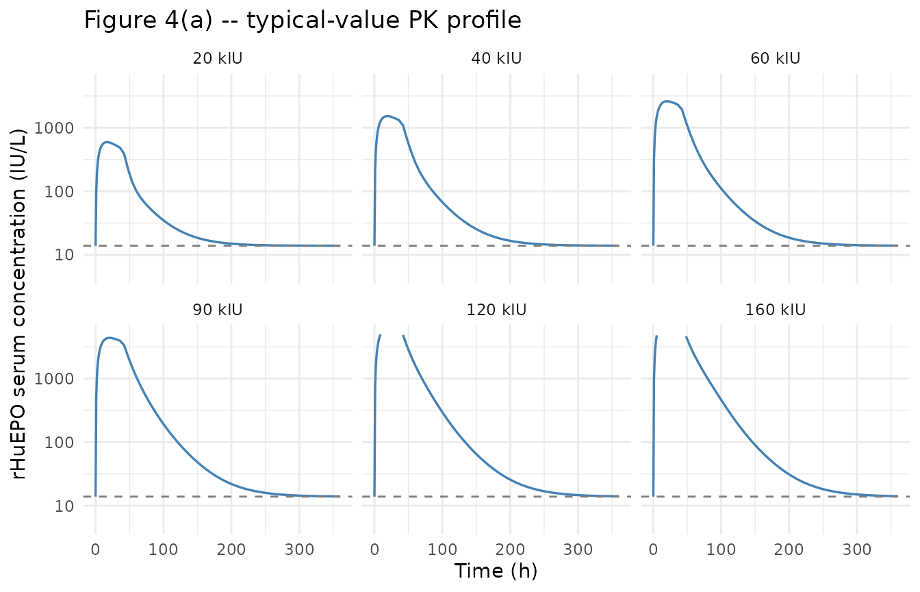
Replicates Figure 4(a) of Perez-Ruixo 2008: median rHuEPO serum concentration vs time, by SC dose.
sim |>
  dplyr::mutate(treatment = factor(treatment, levels = paste0(dose_levels, " kIU")),
                time_d    = time / 24) |>
  ggplot2::ggplot(ggplot2::aes(time_d, RET, group = treatment)) +
  ggplot2::geom_line(color = "firebrick", size = 0.6) +
  ggplot2::geom_hline(yintercept = 1.24, linetype = "dashed", color = "grey50") +
  ggplot2::facet_wrap(~ treatment, ncol = 3) +
  ggplot2::coord_cartesian(xlim = c(0, 30), ylim = c(0, 8)) +
  ggplot2::labs(x = "Time (days)", y = "Reticulocyte count (%)",
                title = "Figure 4(b) -- typical-value reticulocyte response") +
  ggplot2::theme_minimal()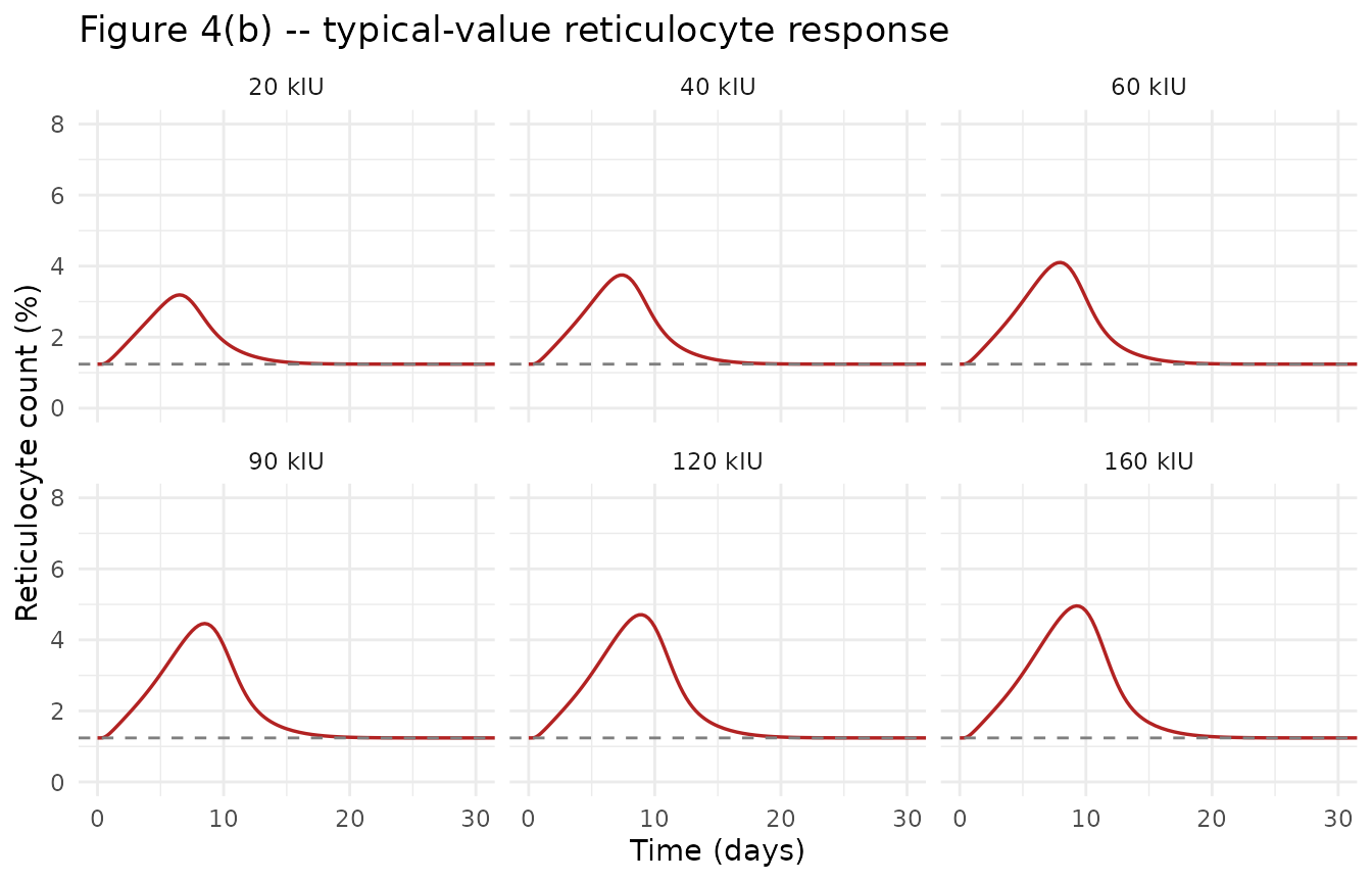
Replicates Figure 4(b) of Perez-Ruixo 2008: median reticulocyte percentage vs time, by SC dose.
peaks <- sim |>
  dplyr::group_by(treatment) |>
  dplyr::summarise(
    Cc_peak       = max(Cc, na.rm = TRUE),
    Cc_peak_t_h   = time[which.max(Cc)],
    RET_peak      = max(RET, na.rm = TRUE),
    RET_peak_t_d  = time[which.max(RET)] / 24,
    .groups = "drop"
  ) |>
  dplyr::mutate(treatment = factor(treatment, levels = paste0(dose_levels, " kIU"))) |>
  dplyr::arrange(treatment)

knitr::kable(
  peaks,
  caption = "Typical-value PK and PD peaks across the six study-C doses.",
  digits  = c(0, 0, 1, 2, 2)
)| treatment | Cc_peak | Cc_peak_t_h | RET_peak | RET_peak_t_d |
|---|---|---|---|---|
| 20 kIU | 593 | 17 | 3.19 | 6.50 |
| 40 kIU | 1520 | 19 | 3.75 | 7.50 |
| 60 kIU | 2606 | 20 | 4.10 | 8.00 |
| 90 kIU | 4374 | 21 | 4.46 | 8.50 |
| 120 kIU | 6228 | 21 | 4.71 | 9.00 |
| 160 kIU | 8768 | 21 | 4.96 | 9.25 |
Validation 3 – mean reticulocyte residence time
Perez-Ruixo 2008 Figure 7(b) reports the mean reticulocyte residence
time MRT_RET(t) (equation 33) for the typical subject at
20, 60 and 160 kIU. Baseline MRT_RET corresponds to the
reciprocal of the baseline reticulocyte aging rate; under rHuEPO the
signal-driven inhibition S0 / SM slows aging and inflates
the residence time, peaking around day 1-2 and decaying back to baseline
as the signal returns to S0.
A faithful reproduction of MRT_RET(t) requires solving the auxiliary ODE of equation 30, which is beyond the scope of this rxode2 simulator vignette (the auxiliary equation depends on the time-varying transfer rate kernel, not on the simulated states). The discussion-section narrative of figure 7 in Perez-Ruixo 2008 is the appropriate reference here.
Validation 4 – signal transduction baseline and saturation
At baseline (C = BSL = 13.9 IU/L), each signal transit compartment
transit_k(0) = sig0 = BSL/(EC50+BSL) = 13.9/(56.3+13.9) = 0.198
(eq 23 implicit form with Smax = 1). Under sustained high exposure
C >> EC50 the signal saturates at 1.0, giving
aging_mod = sig0/1.0 = 0.198 – a ~5-fold slowdown of
reticulocyte aging.
sig0 <- 13.9 / (56.3 + 13.9)
cat("sig0 (baseline signal level):", sig0, "\n")
#> sig0 (baseline signal level): 0.1980057
cat("aging_mod at signal saturation (C >> EC50):", sig0 / 1.0, "\n")
#> aging_mod at signal saturation (C >> EC50): 0.1980057
cat("relative reticulocyte residence-time inflation: ", 1 / (sig0 / 1.0), "x\n", sep = "")
#> relative reticulocyte residence-time inflation: 5.05036x
Assumptions and deviations
-
DOSE covariate. rxode2’s zero-order infusion
absorption (
rate = -2) evaluatespodo()to NA insidef(), so the dose-dependent bioavailabilityF = F0 + Emax(F)*Dose/(ED50(F)+Dose)(Perez-Ruixo 2008 eq 5) is encoded against a user-suppliedDOSEcovariate column rather thanpodo(). The vignette setsDOSEto the same value asamtof the depot/central dose records. The math is identical to the paper. -
Dual-pathway dose timing offset. The depot dose
record is timed at
t_doseand the central dose record att_dose + 1e-3h. rxode2 cannot process two simultaneousrate = -2records at the same time; the picosecond-scale time offset side-steps the collision.alag(central) = tlag2then applies the slow-pathway lag time (~ 2.72 h) so the actual central-compartment administration occurs at ~t_dose + tlag2, exactly as in the paper’s Olsson-Gisleskog 2007 PK structure. -
PK residual error not in this paper. The rHuEPO
concentration residual error (transform-both-sides additive on log
scale, Methods Statistical Model) was not reported in Perez-Ruixo 2008;
its value lives in Olsson-Gisleskog 2007 (the upstream popPK paper, not
on disk for this extraction). The model file encodes
propSd <- fixed(0)per the extraction policy (“If a needed value is unreported, encode fixed(0) + an erratum rather than a class-typical placeholder”). For simulation this means the PK observableCcis delivered without residual noise; the simulator is faithful to the published median PK. -
PD residual error interpretation. Equation 27 is
R_obs = R_pred + epsilonwithepsilon ~ N(0, sigma^2)(additive normal form) and Table II Model D reportssigma = 63.1 %. The “[%]” column header is interpreted here as a proportional CV onR_pred(encoded aspropSd_RET <- 0.631) because the alternative additive reading (sigma = 0.631 % absolute reticulocytes) implies an observation SD about 50 % of the baseline mean, which is implausibly large for the reported data; the proportional reading is the conventional encoding for “[%]”-headered residual columns in popPD tables. - PK priors used (Table I Prior mean column). The PK structural parameters and IIV CV%s are the Olsson-Gisleskog 2007 typical values used as the prior for the MAP-Bayesian POSTHOC PK estimation. The Table I Posterior mean column gives the cohort-mean MAP-Bayesian estimates for the 88 healthy male subjects in this study. The packaged model uses the Prior mean column (the population typical), not the Posterior mean (the cohort empirical mean for this study).
-
fr IIV approximation in the logit domain.
Perez-Ruixo 2008 Methods state that IIV on
frwas modelled with a normal distribution in the logit domain. Table I reportsfr = 60 % (45 %)– a back-transformed- The model encodes
etalogitfr ~ log(0.45^2 + 1) = 0.1854as a log-normal-style approximation on the logit-scale eta; this slightly overestimates the back-transformed CV for large logit shifts but is the standard approximation used across the nlmixr2lib for logit-IIV parameters.
- The model encodes
-
kEPO endogenous-input formulation. The
endogenous-EPO baseline is maintained by a constant input rate kEPO =
CLIBSL + VmaxBSL/(Km+BSL) into the central compartment (paper
eq 4 implicit form), with
central(0) = BSL * vcandperipheral1(0) = BSL * V3setting the pre-dose steady state. After dosing, A2/V2 = total (endogenous + exogenous) EPO concentration and is read directly asCc; no separate additive endogenous term is required at the observation step. - Typical-value RET peak slightly below paper PPC median at higher doses. At 90-160 kIU the typical-value simulation here peaks at 4.5-5.0 % reticulocytes; the paper’s posterior-predictive-check median peaks at ~ 6-7 %. The temporal pattern (peak at day 8-10, dose-ordered rank) matches; the absolute magnitude difference is attributed to the PK trajectory differences between the Olsson- Gisleskog 2007 prior mean (used here) and the cohort-empirical posterior mean (which the paper’s POSTHOC PK predictions used as per-subject inputs to the PD layer). Parameter values were not tuned to close the gap per the extraction policy.
- Smax = 1 in the signal-transduction layer. Perez-Ruixo 2008 Methods state that the maximum signal effect Smax was not identifiable in the presence of the S0/SM ratio, so it is implicitly fixed at 1. The driving function therefore reduces to C/(EC50+C), bounded in [0, 1].
- MRT(t) auxiliary equation not encoded. Figure 7’s reticulocyte mean residence time and figure 6’s reticulocyte residence time distribution rely on the auxiliary ODE of equation 30 (with initial-condition equation 31). They are reported in the paper’s Discussion as additional outputs of Model D rather than as primary observables; this packaged model does not encode the auxiliary equation. The validation here covers the primary observables (Cc and RET) only.