Cenicriviroc (TBR-652) HIV-1 RNA and MCP-1 exposure-response (Marier 2011)
Source:vignettes/articles/Marier_2011_cenicriviroc.Rmd
Marier_2011_cenicriviroc.RmdModel and source
- Citation: Marier JF, Trinh M, Pheng LH, Palleja SM, Martin DE. Pharmacokinetics and pharmacodynamics of TBR-652, a novel CCR5 antagonist, in HIV-1-infected, antiretroviral treatment-experienced, CCR5 antagonist-naive patients. Antimicrob Agents Chemother. 2011;55(6):2768-2774. doi:10.1128/AAC.00713-10. PMCID PMC3101382. PK/PD model form is in Methods ‘Pharmacokinetic/pharmacodynamic modeling’ (p. 2770); the parameter estimates and their standard errors are in Results (p. 2772) and are restated in the Discussion (p. 2773); the fitted curve and the individual data it was fit to are Figure 3 (p. 2773). Companion model file from the same paper: modellib(‘Marier_2011_cenicriviroc_mcp1’).
- Article: https://doi.org/10.1128/AAC.00713-10
- Open-access full text: https://www.ncbi.nlm.nih.gov/pmc/articles/PMC3101382/
Marier et al. (2011) report a double-blind, placebo-controlled,
dose-escalating study of 10 days of once-daily oral monotherapy with the
CCR5 antagonist then known only as TBR-652 in
HIV-1-infected, antiretroviral treatment-experienced,
CCR5-antagonist-naive adults. The compound was later assigned the INN
cenicriviroc; it is a dual CCR5 / CCR2 antagonist, and
this package uses the INN throughout while keeping the development code
visible in each model’s description.
The paper contributes two models, fitted independently on two different biomarkers from the same cohort, so the package carries one file for each:
| Model file | Endpoint | Emax | IC50 |
|---|---|---|---|
Marier_2011_cenicriviroc_hiv1rna |
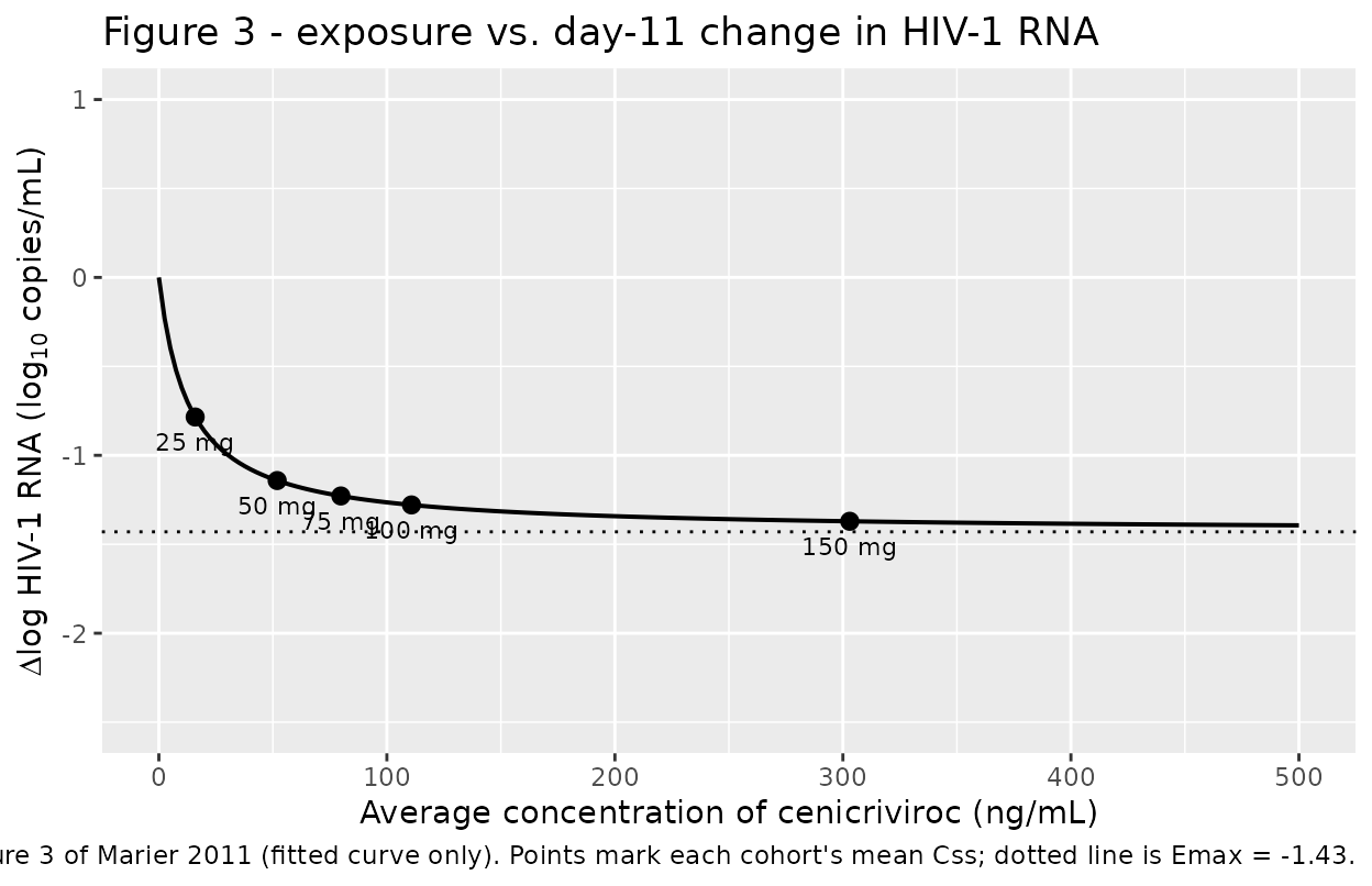
Day-11 change from baseline in plasma HIV-1 RNA | -1.43 log10 copies/mL | 13.1 ng/mL |
Marier_2011_cenicriviroc_mcp1 |
Day-10 change from baseline in plasma MCP-1 | +2.63 log10 pg/mL | 29.8 ng/mL |
Both have the same structural form – a simple, intercept-free, hyperbolic Emax function of the average steady-state cenicriviroc concentration:
Two properties of these models are unusual enough to state up front, because they determine how the rest of this vignette is written.
There is no pharmacokinetic model. Marier 2011
characterised cenicriviroc PK by noncompartmental analysis
only (Methods, “Pharmacokinetics”, p. 2769). There is no
compartmental structure, no CL, no V, no ka to extract. The driving
exposure is therefore supplied to the model as a covariate,
CSS_CVC, rather than generated from dose events – exactly
as for the other static exposure-response models in this library
(Riggs_2012_albinterferon_svr_gt1,
Song_2013_..._dbp,
Mukker_2026_tuvusertib_hERG).
Both models are deterministic. The source reports
two point estimates and their standard errors per endpoint, and nothing
else: no OMEGA, no SIGMA, no residual SD. Neither model carries an eta,
and addSd is fixed(0) in both, so each returns
a single exact curve. Every check below is consequently an exact
numerical identity rather than a statistic over a simulated cohort, and
is asserted at correspondingly tight tolerance.
mod_hiv  <- readModelDb("Marier_2011_cenicriviroc_hiv1rna")
mod_mcp1 <- readModelDb("Marier_2011_cenicriviroc_mcp1")

# Both models are static: no ODE states, no dose events. The event table is
# therefore a plain observation frame carrying the driving covariate, with
# cmt = NA_character_ because there is no compartment to point at. This is the
# same idiom used by Mukker_2026_tuvusertib_QTc.Rmd.
#
# NOTE on the muffled warning: rxode2 emits "multi-subject simulation without
# 'omega'" on every solve here. That is expected and correct -- these models
# have no random effects, so there is no omega to supply. Passing `omega = NA`
# is NOT the fix: for a model that declares no eta, rxode2 evaluates
# dim(NA)[1] and fails with "rep(0, dim(.omega)[1]) : invalid 'times'
# argument". Only that one message is muffled; any other warning propagates.
solve_static <- function(mod, css) {
  ev <- data.frame(
    id      = seq_along(css),
    CSS_CVC = css,
    time    = 0,
    evid    = 0,
    amt     = 0,
    cmt     = NA_character_
  )
  withCallingHandlers(
    as.data.frame(rxode2::rxSolve(mod, events = ev)),
    warning = function(w) {
      if (grepl("without.*'omega'", conditionMessage(w))) {
        invokeRestart("muffleWarning")
      }
    }
  )
}
Population
The study (protocol 652-2-201) screened and entered 54 patients at 10 sites, 9 in the United States and 1 in Argentina. Approximately 10 patients per dose level were randomised 4:1 to cenicriviroc or matching placebo at 25, 50, 75, 100 and 150 mg once daily for 10 days, followed by a 40-day observation period.
From Table 1 (p. 2770): 87% male (7 of 54 female); mean age 38.9 years (SD 7.95), inclusion range 18-65; mean weight 79.81 kg (SD 17.08); mean height 176.71 cm (SD 9.685); mean BMI 25.65 kg/m^2 (SD 5.322). Race and ethnicity were 55.6% Caucasian, 25.9% African-American, 13.0% Hispanic, 1.9% Asian and 3.7% other.
Entry required treatment experience with all antiretroviral therapy stopped at least 6 weeks earlier (actual time off therapy ranged from 6 weeks to 3 years), no prior CCR5-antagonist exposure, CCR5-tropic virus by the enhanced-sensitivity Trofile assay, plasma HIV-1 RNA of at least 5,000 copies/mL and a CD4+ count of at least 250 cells/mm^3.
Two per-patient reassignments the paper makes explicitly matter for
the denominators. Patient 2007 was randomised to the 50 mg cohort but
mistakenly received 25 mg and was analysed with the 25 mg cohort.
Patient 5002, in the 150 mg cohort, was retrospectively found to harbour
predominantly CXCR4-tropic virus at baseline, was therefore ineligible,
and was omitted from the antiviral efficacy analyses. The HIV-1 RNA
analysis set used here is consequently 42 treated plus 10 placebo
patients; the paper states no analysis-set size for the MCP-1 model, so
n_subjects is left NA in that file rather than
guessed.
The same information is available programmatically:
pop <- rxode2::rxode(mod_hiv)$population
str(pop[c("species", "n_subjects", "disease_state", "endpoint")])
#> List of 4
#>  $ species      : chr "human"
#>  $ n_subjects   : int 52
#>  $ disease_state: chr "HIV-1 infection, antiretroviral treatment-experienced but off all antiretroviral therapy for at least 6 weeks ("| __truncated__
#>  $ endpoint     : chr "Change from baseline (day 1 predose) in plasma HIV-1 RNA on day 11, in log10 copies/mL. Assayed with the Cobas "| __truncated__
Source trace
Every value below is recorded as an in-file comment beside its
ini() entry in
inst/modeldb/specificDrugs/Marier_2011_cenicriviroc_hiv1rna.R
and ..._mcp1.R. This table collects them for review. Page
numbers refer to the journal pagination (the article runs
pp. 2768-2774).
| Model | Parameter / equation | Value | Source location |
|---|---|---|---|
| both | E = emax * Css / (ic50 + Css) |
n/a | Methods, “Pharmacokinetic/pharmacodynamic modeling”, p. 2770; selection by AIC stated in Results, p. 2772 |
| hiv1rna | emax |
-1.43 log10 copies/mL | Results p. 2772; restated Discussion p. 2773 and Abstract |
| hiv1rna | SE(emax) |
0.138 log10 copies/mL | Results p. 2772 |
| hiv1rna |
lic50 = log(13.1) |
13.1 ng/mL | Results p. 2772; restated Discussion p. 2773 |
| hiv1rna | SE(ic50) |
6.53 ng/mL | Results p. 2772 |
| hiv1rna | addSd |
fixed(0) |
not reported; see Assumptions |
| mcp1 | emax |
+2.63 log10 pg/mL | Results pp. 2772-2773 |
| mcp1 | SE(emax) |
0.233 log10 pg/mL | Results p. 2773 |
| mcp1 |
lic50 = log(29.8) |
29.8 ng/mL | Results pp. 2772-2773 |
| mcp1 | SE(ic50) |
9.45 ng/mL | Results p. 2773 |
| mcp1 | addSd |
fixed(0) |
not reported; see Assumptions |
| both |
CSS_CVC definition (AUC0-24 / 24 h) |
see Table 2 | Methods, “Pharmacokinetics”, p. 2769; values Table 2, p. 2772 |
| hiv1rna | fitted curve + individual data | n/a | Figure 3, p. 2773 |
| mcp1 | fitted curve + individual data | n/a | Figure 4, p. 2773 |
| hiv1rna | observed day-11 medians | Table 3, p. 2772 |
Units
Because the observation of each model is a change on a log scale rather than a concentration, the dimensional bookkeeping is worth writing out explicitly.
| Symbol | Units | Note |
|---|---|---|
CSS_CVC |
ng/mL | total (not unbound) plasma cenicriviroc |
ic50 |
ng/mL | same basis as CSS_CVC, so the ratio is
dimensionless |
CSS_CVC / (ic50 + CSS_CVC) |
dimensionless | fraction of maximal effect, in [0, 1) |
emax (hiv1rna) |
log10 copies/mL | signed; negative = viral suppression |
emax (mcp1) |
log10 pg/mL | signed; positive = MCP-1 accumulation |
d_viral_load |
log10 copies/mL | change from baseline; add baseline to get an absolute level |
dmcp1 |
log10 pg/mL | change from baseline, i.e. a log10 fold-change |
The product of a dimensionless fraction with emax
therefore carries emax’s units, which is what each model’s
units$concentration declares. Note that neither model
carries a baseline, so neither can produce an absolute HIV-1 RNA or
MCP-1 concentration on its own.
Structural verification
Three exact identities are checked first. They are algebraic consequences of the encoding, so they are asserted at machine precision.
chk_hiv  <- solve_static(mod_hiv,  c(0, 13.1))
chk_mcp1 <- solve_static(mod_mcp1, c(0, 29.8))

stopifnot(
  # 1. No intercept: at zero exposure (placebo) both models return exactly 0.
  #    This is the property Figure 3 and Figure 4 show graphically, with the
  #    placebo subjects sitting on the origin.
  chk_hiv$d_viral_load[1]  == 0,
  chk_mcp1$dmcp1[1]      == 0,

  # 2. The reported IC50 really is the half-maximal concentration: at
  #    Css = IC50 each model returns exactly emax / 2.
  isTRUE(all.equal(chk_hiv$d_viral_load[2], -1.43 / 2, tolerance = 1e-12)),
  isTRUE(all.equal(chk_mcp1$dmcp1[2],      2.63 / 2, tolerance = 1e-12)),

  # 3. Residual error really is switched off: the simulated observation
  #    equals the individual prediction exactly, confirming addSd = fixed(0).
  isTRUE(all.equal(chk_hiv$sim,  chk_hiv$d_viral_load,  tolerance = 1e-12)),
  isTRUE(all.equal(chk_mcp1$sim, chk_mcp1$dmcp1,      tolerance = 1e-12))
)

# The signs are opposite and that is the point: CCR5 blockade suppresses virus,
# CCR2 blockade lets the receptor's own ligand accumulate.
stopifnot(chk_hiv$d_viral_load[2] < 0, chk_mcp1$dmcp1[2] > 0)
The exposure metric: Css = AUC0-24 / 24 h
The models consume an NCA-derived quantity, so the first validation
is of that quantity rather than of the model. Marier 2011 defines
Css as the average concentration under steady-state
conditions and computes AUC0-24 by the linear trapezoidal rule (Methods,
p. 2769). Table 2 reports both, which makes the definition checkable
against the paper’s own numbers.
This is why the vignette carries no PKNCA section. PKNCA validates a simulated concentration-time profile against a published NCA table; here the published NCA table is the model’s input, and there is no PK model to generate a profile from. The identity below is the corresponding check that is actually meaningful.
tab2 <- tibble::tribble(
  ~dose_mg, ~auc0_24, ~css_reported, ~cmax,  ~cmin,  ~tmax, ~thalf, ~cl_f,
        25,    382.0,         15.92,  35.11,  6.883,  2.98,  22.50,  81.31,
        50,   1245.0,         51.89, 102.40, 21.470,  4.00,  47.62,  49.26,
        75,   1916.0,         79.82, 157.00, 30.060,  3.50,  29.78,  42.17,
       100,   2659.0,        110.80, 196.50, 30.000,  4.00,  32.06,  48.06,
       150,   7272.0,        303.00, 508.10, 128.000, 4.00,  41.26,  22.95
) |>
  dplyr::mutate(
    css_derived = auc0_24 / 24,
    pct_diff    = 100 * (css_derived - css_reported) / css_reported
  )

# Deterministic arithmetic on transcribed table values -- no simulation, no RNG.
# The residue is pure rounding of the 4-significant-figure printed AUC and Css,
# so the bound is tight on purpose: anything larger means a mis-transcription.
stopifnot(max(abs(tab2$pct_diff)) < 0.05)

tab2 |>
  dplyr::select(dose_mg, auc0_24, css_reported, css_derived, pct_diff) |>
  dplyr::rename(
    "Dose (mg QD)"          = dose_mg,
    "AUC0-24 (ng*h/mL)"     = auc0_24,
    "Css reported (ng/mL)"  = css_reported,
    "AUC0-24 / 24 (ng/mL)"  = css_derived,
    "Difference (%)"        = pct_diff
  ) |>
  knitr::kable(
    digits  = c(0, 1, 2, 3, 4),
    caption = "Table 2 of Marier 2011: the reported Css is exactly AUC0-24 / 24 h."
)| Dose (mg QD) | AUC0-24 (ng*h/mL) | Css reported (ng/mL) | AUC0-24 / 24 (ng/mL) | Difference (%) |
|---|---|---|---|---|
| 25 | 382 | 15.92 | 15.917 | -0.0209 |
| 50 | 1245 | 51.89 | 51.875 | -0.0289 |
| 75 | 1916 | 79.82 | 79.833 | 0.0167 |
| 100 | 2659 | 110.80 | 110.792 | -0.0075 |
| 150 | 7272 | 303.00 | 303.000 | 0.0000 |
Reproducing the paper’s published percentages of Emax
This is the sharpest available check on the HIV-1 RNA model, and it is worth spelling out why. Results (p. 2772) states:
Based on the PK/PD model, the average steady-state concentration levels of TBR-652 for the 25-, 50-, 75-, 100-, and 150-mg doses are expected to result in 54.5%, 79.6%, 85.7%, 89.3%, and 95.8% of the maximum inhibitory effect (Emax) of TBR-652, respectively.
That single row simultaneously pins down four things that would
otherwise be assumptions: the driver (Css,
not AUC0-24 and not Cmax, both of which the Methods say were tested),
the IC50 (13.1 ng/mL), the absence of a Hill
coefficient, and the absence of an intercept.
No other combination reproduces it.
emax_hiv <- -1.43

pct <- tab2 |>
  dplyr::transmute(
    dose_mg,
    css        = css_reported,
    paper_pct  = c(54.5, 79.6, 85.7, 89.3, 95.8),
    model_pct  = 100 * solve_static(mod_hiv, css_reported)$d_viral_load / emax_hiv,
    diff_pp    = model_pct - paper_pct
  )

# Deterministic: a fixed curve evaluated at five transcribed concentrations.
# The residue is 0.06-0.36 percentage points and is explained by the paper
# averaging PER-SUBJECT percentages while this evaluates at the cohort MEAN
# Css -- Jensen's inequality on a concave function, which must bias the
# per-subject average DOWNWARD, and does, at every one of the five doses.
# A wrong IC50, a wrong driver or a stray Hill term moves these by whole
# percentage points, so 0.5 still goes red on any of those.
stopifnot(max(abs(pct$diff_pp)) < 0.5)

# Direction of the residue is itself informative and is deterministic here
# (no cohort, no RNG), so it can be asserted exactly.
stopifnot(all(pct$diff_pp > 0))

pct |>
  dplyr::rename(
    "Dose (mg QD)"        = dose_mg,
    "Css (ng/mL)"         = css,
    "Paper % of Emax"     = paper_pct,
    "Model % of Emax"     = model_pct,
    "Difference (pp)"     = diff_pp
  ) |>
  knitr::kable(
    digits  = c(0, 2, 1, 2, 3),
    caption = "Marier 2011 Results p. 2772, reproduced from the packaged model."
)| Dose (mg QD) | Css (ng/mL) | Paper % of Emax | Model % of Emax | Difference (pp) |
|---|---|---|---|---|
| 25 | 15.92 | 54.5 | 54.86 | 0.359 |
| 50 | 51.89 | 79.6 | 79.84 | 0.243 |
| 75 | 79.82 | 85.7 | 85.90 | 0.202 |
| 100 | 110.80 | 89.3 | 89.43 | 0.127 |
| 150 | 303.00 | 95.8 | 95.86 | 0.056 |
Replicate published figures
# Replicates Figure 3 of Marier 2011: fitted Emax curve of the day-11 change
# from baseline in HIV-1 RNA against average steady-state concentration.
# The published figure spans 0-500 ng/mL on the x-axis and +1.0 to -2.5 on the
# y-axis; the individual patient data it overlays are not publicly available,
# so only the fitted curve is reproduced, with the cohort mean Css marked.
css_grid <- seq(0, 500, length.out = 200)

curve_hiv <- solve_static(mod_hiv, css_grid)

cohort_hiv <- solve_static(mod_hiv, tab2$css_reported) |>
  dplyr::mutate(dose = paste0(tab2$dose_mg, " mg"))

ggplot(curve_hiv, aes(CSS_CVC, d_viral_load)) +
  geom_hline(yintercept = emax_hiv, linetype = "dotted") +
  geom_line(linewidth = 0.7) +
  geom_point(data = cohort_hiv, size = 2.4) +
  geom_text(
    data = cohort_hiv, aes(label = dose),
    vjust = 1.9, size = 3
  ) +
  scale_y_continuous(limits = c(-2.5, 1.0)) +
  labs(
    x       = "Average concentration of cenicriviroc (ng/mL)",
    y       = expression(Delta*"log HIV-1 RNA (log"[10]*" copies/mL)"),
    title   = "Figure 3 - exposure vs. day-11 change in HIV-1 RNA",
    caption = paste(
      "Replicates Figure 3 of Marier 2011 (fitted curve only).",
      "Points mark each cohort's mean Css; dotted line is Emax = -1.43."
    )
  )
# Replicates Figure 4 of Marier 2011: fitted Emax curve of the change from
# baseline in plasma MCP-1 against average steady-state concentration.
# Published axes: 0-500 ng/mL and 0.0-3.0.
curve_mcp1 <- solve_static(mod_mcp1, css_grid)

cohort_mcp1 <- solve_static(mod_mcp1, tab2$css_reported) |>
  dplyr::mutate(dose = paste0(tab2$dose_mg, " mg"))

ggplot(curve_mcp1, aes(CSS_CVC, dmcp1)) +
  geom_hline(yintercept = 2.63, linetype = "dotted") +
  geom_line(linewidth = 0.7) +
  geom_point(data = cohort_mcp1, size = 2.4) +
  geom_text(
    data = cohort_mcp1, aes(label = dose),
    vjust = -1.1, size = 3
  ) +
  scale_y_continuous(limits = c(0, 3.0)) +
  labs(
    x       = "Average concentration of cenicriviroc (ng/mL)",
    y       = expression(Delta*"log plasma MCP-1 (log"[10]*" pg/mL)"),
    title   = "Figure 4 - exposure vs. change in plasma MCP-1",
    caption = paste(
      "Replicates Figure 4 of Marier 2011 (fitted curve only).",
      "Points mark each cohort's mean Css; dotted line is Emax = +2.63."
    )
  )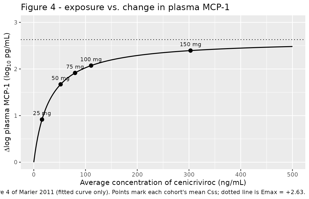
The published Figure 4 curve reaches roughly 2.47 at the right-hand edge of the plotted concentration range. That is a readable feature of the figure rather than a printed number, so it is checked loosely, as a shape check on the plateau:
plateau <- solve_static(mod_mcp1, 490)$dmcp1

# Deterministic curve evaluation. 2.479 is the exact value; the window admits
# the imprecision of reading an asymptote off a printed figure, while still
# failing if Emax or IC50 were mis-transcribed (which would move it by >0.3).
stopifnot(plateau > 2.35, plateau < 2.60)
round(plateau, 3)
#> [1] 2.479
Comparison against the published observed medians
Table 3 (p. 2772) reports the observed median day-11 change from baseline in each cohort. The model was fit to individual patients rather than to these medians, and the medians carry the placebo response (+0.1 log10 copies/mL) and the 100 mg cohort’s distinct F2 tablet formulation, neither of which the model represents. This comparison is therefore a plausibility check, not an identity.
obs_cmp <- tibble::tibble(
  dose_mg       = tab2$dose_mg,
  css           = tab2$css_reported,
  observed      = c(-0.5, -1.3, -1.6, -1.2, -1.5),
  predicted     = solve_static(mod_hiv, tab2$css_reported)$d_viral_load
) |>
  dplyr::mutate(residual = predicted - observed)

# Deterministic (transcribed medians vs a fixed curve), but the two sides
# differ by a real mechanism -- cohort median vs individual-level fit, plus an
# unmodelled placebo response and formulation effect -- so this is bounded on
# the CENTRE and on magnitude, not on any single cohort's extreme.
stopifnot(
  abs(mean(obs_cmp$residual)) < 0.25,
  max(abs(obs_cmp$residual))  < 0.60
)

obs_cmp |>
  dplyr::rename(
    "Dose (mg QD)"                        = dose_mg,
    "Css (ng/mL)"                         = css,
    "Observed median (log10 copies/mL)"   = observed,
    "Model prediction (log10 copies/mL)"  = predicted,
    "Residual"                            = residual
  ) |>
  knitr::kable(
    digits  = c(0, 2, 2, 3, 3),
    caption = "Marier 2011 Table 3 day-11 medians vs. the packaged model at each cohort's mean Css."
)| Dose (mg QD) | Css (ng/mL) | Observed median (log10 copies/mL) | Model prediction (log10 copies/mL) | Residual |
|---|---|---|---|---|
| 25 | 15.92 | -0.5 | -0.784 | -0.284 |
| 50 | 51.89 | -1.3 | -1.142 | 0.158 |
| 75 | 79.82 | -1.6 | -1.228 | 0.372 |
| 100 | 110.80 | -1.2 | -1.279 | -0.079 |
| 150 | 303.00 | -1.5 | -1.371 | 0.129 |
The largest residual is at 75 mg, where the observed median (-1.6) is the deepest of any cohort while its mean Css sits mid-range. The model, being monotone in exposure, cannot reproduce a non-monotone dose-median sequence (-0.5, -1.3, -1.6, -1.2, -1.5); the authors attribute the 100 mg dip to the F2 formulation, and the 75 mg and 150 mg cohorts differ by only 0.1 log10 in observed median despite a nearly 4-fold difference in exposure, which is exactly the saturation the Emax model encodes.
Parameter precision
The standard errors reported alongside the point estimates are worth carrying into the vignette, because they differ sharply between the two parameters and that difference is interpretable.
prec <- tibble::tribble(
  ~model,     ~parameter, ~estimate, ~se,
  "hiv1rna",  "Emax",         -1.43, 0.138,
  "hiv1rna",  "IC50",         13.10, 6.530,
  "mcp1",     "Emax",          2.63, 0.233,
  "mcp1",     "IC50",         29.80, 9.450
) |>
  dplyr::mutate(
    rse_pct = 100 * se / abs(estimate),
    ci_lo   = estimate - 1.96 * se,
    ci_hi   = estimate + 1.96 * se
  )

# A Wald interval must bracket its own point estimate -- a cheap guard against
# a transposed SE or a sign-mangled estimate (the PDF-glyph hazard noted in the
# model files). Deterministic arithmetic, so exact.
stopifnot(all(prec$ci_lo < prec$estimate), all(prec$estimate < prec$ci_hi))

# Both Emax parameters are well determined; both IC50s are not. Assert the
# ordering that the paper's own numbers imply.
stopifnot(
  prec$rse_pct[prec$parameter == "Emax"] < 15,
  prec$rse_pct[prec$parameter == "IC50"] > 25
)

prec |>
  dplyr::rename(
    "Model"           = model,
    "Parameter"       = parameter,
    "Estimate"        = estimate,
    "SE"              = se,
    "RSE (%)"         = rse_pct,
    "Wald 95% lower"  = ci_lo,
    "Wald 95% upper"  = ci_hi
  ) |>
  knitr::kable(
    digits  = c(0, 0, 2, 3, 1, 3, 3),
    caption = "Point estimates and standard errors as reported in Marier 2011 Results."
)| Model | Parameter | Estimate | SE | RSE (%) | Wald 95% lower | Wald 95% upper |
|---|---|---|---|---|---|---|
| hiv1rna | Emax | -1.43 | 0.138 | 9.7 | -1.700 | -1.160 |
| hiv1rna | IC50 | 13.10 | 6.530 | 49.8 | 0.301 | 25.899 |
| mcp1 | Emax | 2.63 | 0.233 | 8.9 | 2.173 | 3.087 |
| mcp1 | IC50 | 29.80 | 9.450 | 31.7 | 11.278 | 48.322 |
The HIV-1 RNA IC50 has an RSE of 49.8% and a Wald lower
bound of 0.30 ng/mL – positive, but only just. This is a structural
consequence of the study design rather than a transcription problem:
only the 25 mg cohort (mean Css 15.92 ng/mL) sits anywhere near 13.1
ng/mL, and every other cohort is on the plateau. The data constrain the
maximum effect far better than the potency. Any use of this model to
extrapolate to sub-25 mg doses should carry that caveat.
Cross-model comparison
ic50_hiv  <- 13.1
ic50_mcp1 <- 29.8

# Deterministic ratio of two printed constants.
stopifnot(isTRUE(all.equal(ic50_mcp1 / ic50_hiv, 2.275, tolerance = 1e-3)))

tibble::tibble(
  `Dose (mg QD)`             = tab2$dose_mg,
  `Css (ng/mL)`              = tab2$css_reported,
  `% of antiviral Emax`      = 100 * tab2$css_reported / (ic50_hiv  + tab2$css_reported),
  `% of MCP-1 Emax`          = 100 * tab2$css_reported / (ic50_mcp1 + tab2$css_reported)
) |>
  knitr::kable(
    digits  = c(0, 2, 1, 1),
    caption = "CCR5-mediated antiviral effect saturates at lower exposure than CCR2-mediated MCP-1 accumulation."
)| Dose (mg QD) | Css (ng/mL) | % of antiviral Emax | % of MCP-1 Emax |
|---|---|---|---|
| 25 | 15.92 | 54.9 | 34.8 |
| 50 | 51.89 | 79.8 | 63.5 |
| 75 | 79.82 | 85.9 | 72.8 |
| 100 | 110.80 | 89.4 | 78.8 |
| 150 | 303.00 | 95.9 | 91.0 |
The MCP-1 IC50 is 2.3-fold higher than the antiviral
IC50, i.e. more cenicriviroc exposure is needed for
half-maximal CCR2 blockade than for half-maximal CCR5-mediated viral
suppression. That ordering is consistent with the in-vitro potencies the
paper quotes in its Introduction (p. 2768) and with the authors’ reading
that the MCP-1 plateau is reached only at the exposures associated with
the 150 mg dose.
For orientation, the Discussion (p. 2773) compares the antiviral
parameters against maraviroc, the first approved CCR5 antagonist, for
which 10 days of 100-300 mg dosing gave Emax values of -1.13 to -1.45
log10 copies/mL and an IC50 of 8 ng/mL. Cenicriviroc’s -1.43 log10
copies/mL and 13.1 ng/mL sit inside and just above those, respectively.
That comparator model is packaged separately as
Davis_2008_maraviroc – note, however, that the Davis model
is a concentration-QT analysis, not the antiviral exposure-response the
Discussion cites (which is reference 13 of Marier 2011 and was not
available when this model was built), so the two are not directly
comparable and no cross-check is attempted.
Assumptions and deviations
No pharmacokinetic model exists in the source. Marier 2011 analysed cenicriviroc PK by noncompartmental methods only. The models therefore consume
CSS_CVCas a covariate and cannot be driven from a dose. To simulate a dose, supplyCssexternally, or approximate it asDose / (CL/F * 24 h)using the cohort mean CL/F values in Table 2 – but note that CL/F is not constant over the studied range (81.31, 49.26, 42.17, 48.06 and 22.95 L/h at 25 to 150 mg QD), exposure rose more than dose-proportionally at 150 mg, and two patients dosed in Argentina showed more than 2-fold higher exposure than the rest of their cohort, which the authors attribute to a possible high-fat food effect. A single clearance value will misstate Css outside 50-100 mg.No inter-individual variability and no residual error are reported, for either endpoint. The source publishes two point estimates and two standard errors per model and nothing else. Figures 3 and 4 show clear residual scatter (roughly +/- 0.5 log10 units about each curve), but no estimate of it is given, so none is invented:
addSdisfixed(0)in both files and each model returns the deterministic curve. Re-fitting either model to new data requires supplying a residual-error estimate.Neither model carries a baseline. Both outputs are changes from baseline.
d_viral_loadmust be added to a subject’s baseline log10 HIV-1 RNA to obtain an absolute day-11 level;dmcp1is a log10 fold-change, so an absolute MCP-1 concentration isbaseline * 10^dmcp1. The paper reports baseline HIV-1 RNA by cohort (Table 3 medians 4.0-4.6 log10 copies/mL) but reports no baseline MCP-1 concentration at all, so the MCP-1 model cannot be converted to absolute concentrations from the available information.Drug naming. The source names the compound only as TBR-652 (also TAK-652). The files use the INN cenicriviroc per the library’s generic-name-over- development-code policy, with the development code retained in each
descriptionand in this vignette so the paper remains findable.The model form is inferred from prose plus a numeric check, not from a printed equation. Marier 2011 never writes the Emax equation out. Methods (p. 2770) says a maximum-inhibitory-effect model “with and without sigmoidal factor (gamma)” and linear models were tested against AUC0-24, Cmax and Css, and Results (p. 2772) says the simple Emax model was selected by AIC. The specific form encoded here – hyperbolic, no Hill term, no intercept, driven by Css – is fixed by three independent confirmations: it reproduces the paper’s own published percentages of Emax to within 0.36 percentage points at all five doses (checked above), the fitted curves in Figures 3 and 4 both pass through the origin, and the observed placebo change was +0.1 log10 copies/mL, leaving no placebo effect to model. No alternative form reproduces the percentage row.
Sign of the MCP-1 Emax. The MCP-1
Emaxis printed without a sign (2.63 log10) immediately adjacent to a sibling parameter that is negative, which is precisely the situation in which a dropped minus sign hides. It is confirmed positive three ways: the raw PDF text layer preserves minus-sign glyphs on every occurrence of the -1.43 antiviral Emax and shows none before 2.63; Figure 4’s y-axis runs 0.0 to 3.0 with no negative region and its curve rises; and the mechanism requires it, since blocking CCR2 blocks the clearance route of its own ligand.Two new canonical PD-output names were registered for this extraction, both as members of the existing change-from-baseline PD-output family documented at
ddbp/dsbp/tmccfbininst/references/compartment-names.md:d_viral_load(the change-from-baseline sibling of the existing absoluteviral_loadstate, on the same pattern asddbp/dbp) anddmcp1. A new covariate canonicalCSS_CVCwas registered as a member of the documentedCSS_<DRUG>family alongsideCSS_RBV,CSS_ALBIFNandCSS_DFO; it differs from those three in being noncompartmental in origin rather than derived from an upstream population PK fit.No PKNCA section. There is no simulated concentration-time profile to integrate, because there is no PK model. The paper’s NCA table is this model’s input rather than something it can reproduce; the corresponding meaningful check – that the reported
Cssreally isAUC0-24 / 24 h– is done above instead.n_subjectsdiffers between the two files. The HIV-1 RNA file records 52 (42 treated per the day-11 row of Table 3, plus 10 placebo). The MCP-1 file recordsNA: the paper states no analysis-set size for that endpoint, and counting points off Figure 4 would be a guess.Covariates are documented but unused. Weight, age and sex are tabulated in Table 1 but never entered into either PK/PD model, and the paper reports no covariate screen on the Emax parameters. They are recorded in
covariatesDataExcludedin both files so the provenance is preserved without implying an effect that was never estimated.