Doripenem (Nonoshita 2020)
Source:vignettes/articles/Nonoshita_2020_doripenem.Rmd
Nonoshita_2020_doripenem.RmdModel and source
- Citation: Nonoshita K, Suzuki Y, Tanaka R, Kaneko T, Ohchi Y, Sato Y, Yasuda N, Goto K, Kitano T, Itoh H. Population pharmacokinetic analysis of doripenem for Japanese patients in intensive care unit. Sci Rep. 2020;10:22148. doi:10.1038/s41598-020-79076-6
- Description: Two-compartment IV population PK model for doripenem in 21 Japanese adult intensive care unit patients, 9 of them on continuous renal replacement therapy (continuous hemodiafiltration) (Nonoshita 2020). Total clearance is the sum of a body clearance and, when CRRT is running, a CRRT clearance fixed to the filtrate (effluent) flow rate times the 0.919 unbound fraction of doripenem. Body clearance is estimated separately for the CRRT and non-CRRT strata, each with its own power effect of Cockcroft-Gault creatinine clearance centred on its own stratum median (52.75 and 62.25 mL/min). Body weight and serum albumin were screened but not retained.
- Article: Sci Rep. 2020;10:22148 (open access)
Read the “Assumptions and deviations” section before using this model. The parameter values below are transcribed exactly as the paper prints them, but they predict roughly twice the plasma concentrations that the paper’s own visual predictive check and goodness-of-fit plots show for the same 500 mg dose. The comparison is in the “Visual predictive check” section.
Population
Twenty-one adult inpatients in the intensive care unit of Oita University Hospital, Japan, treated with doripenem for severe infection (bacteremia, sepsis or septic shock, infective endocarditis, pneumonia, intraperitoneal or urinary-tract infection, postoperative infection). There were 18 men and 3 women, age 61.8 +/- 18.9 years (range 15-86), body weight 61.5 +/- 13.6 kg (range 28.8-92.4), APACHE II 17.6 +/- 6.7 and SOFA 7.5 +/- 2.6 (Table 1 and Supplementary Table S1). Cockcroft-Gault creatinine clearance was 68.0 +/- 33.4 mL/min (range 20.7-155.6).
Nine patients were on continuous renal replacement therapy (CRRT), given as continuous hemodiafiltration through a cellulose triacetate membrane with a blood flow of 80-100 mL/min, dialysate and replacement-fluid flows of 0.3-0.9 L/h each, and a filtrate flow (QE) of 0.6-1.8 L/h. Creatinine clearance was 57.3 +/- 26.5 mL/min in the CRRT stratum and 76.0 +/- 35.8 mL/min in the other 12 patients.
Twenty patients received 500 mg and one received 250 mg as a 1 h infusion. Plasma was sampled before and 1, 2, 4, 6 and 8 h after the start of the first infusion only (97 samples).
The same information is available programmatically via the model’s
population metadata
(readModelDb("Nonoshita_2020_doripenem")()$population).
Source trace
The per-parameter origin is recorded as an in-file comment next to
each ini() entry in
inst/modeldb/specificDrugs/Nonoshita_2020_doripenem.R. The
table below collects them in one place for review.
| Equation / parameter | Value | Source location |
|---|---|---|
Two-compartment model, IV infusion, CL_body and
CL_CRRT both from the central compartment |
n/a | Methods “Population pharmacokinetics”; Figure 1 |
CL_total = CL_body(non-CRRT) = 3.65 x (Ccr/62.25)^0.64
without CRRT |
n/a | Abstract; Results “final model” paragraph |
CL_total = CL_body(CRRT) + CL_CRRT = 2.49 x (Ccr/52.75)^0.42 + CL_CRRT
with CRRT |
n/a | Abstract; Results “final model” paragraph |
CL_CRRT = QE x 0.919 |
n/a | Abstract; Results “final model” paragraph |
lcl_offcrrt |
3.65 L/h | Table 3, population mean |
lcl_oncrrt |
2.49 L/h | Table 3, population mean |
lvc |
10.04 L | Table 3, population mean |
lvp |
8.13 L | Table 3, population mean |
lq |
3.53 L/h | Table 3, population mean |
e_crcl_cl_offcrrt |
0.64 | Results final-model equation |
e_crcl_cl_oncrrt |
0.42 | Results final-model equation |
fu |
0.919 (fixed, from the literature) | Results final-model equation (Hori 2006) |
| CRCL centring values | 62.25 and 52.75 mL/min (stratum medians) | Results final-model equation; Discussion |
etalcl_offcrrt |
7.3% CV -> 0.0053149 | Table 3; Discussion |
etalcl_oncrrt |
22.2% CV -> 0.048108 | Table 3; Discussion |
etalvc |
13.2% CV -> 0.017274 | Table 3; Results |
etalvp |
24.2% CV -> 0.056913 | Table 3; Results |
etalq |
12.7% CV -> 0.016000 | Table 3; Results |
addSd |
0.70 mg/L | Table 3, residual variability estimate |
propSd |
0.365 | Table 3; Results “residual variability was 36.5%” |
Inter-individual variability was modelled exponentially (Methods), so
each percentage is converted with
omega^2 = log(CV^2 + 1).
Typical-value checks
The model is deterministic in the typical subject, so the paper’s
clearance arithmetic can be checked exactly. The Discussion reports that
the nine CRRT patients had a total clearance of 3.81 L/h and a CRRT
clearance of 1.31 L/h (means of the individual estimates). At the
CRRT-stratum median creatinine clearance of 52.75 mL/min the body
clearance is the typical 2.49 L/h, and a CRRT clearance of 1.31 L/h
corresponds to a filtrate flow of 1.31 / 0.919 = 1.43 L/h,
inside the 0.6-1.8 L/h range the Methods report.
mod <- rxode2::rxode2(readModelDb("Nonoshita_2020_doripenem"))
#> ℹ parameter labels from comments will be replaced by 'label()'
mod_typ <- rxode2::zeroRe(mod)

typ_cov <- tibble::tribble(
  ~scenario,                                ~RRT_CRRT_STATUS, ~CRCL, ~RRT_CRRT_EFFLUENT_FLOW,
  "No CRRT, CRCL 62.25 mL/min",                           0,  62.25,                       0,
  "CRRT, CRCL 52.75 mL/min, QE 0.6 L/h",                  1,  52.75,                     600,
  "CRRT, CRCL 52.75 mL/min, QE 1.43 L/h",                 1,  52.75,           1310 / 0.919,
  "CRRT, CRCL 52.75 mL/min, QE 1.8 L/h",                  1,  52.75,                    1800
) |>
  dplyr::mutate(id = dplyr::row_number())

ev_typ <- rxode2::et(amt = 500, dur = 1, cmt = "central") |>
  rxode2::et(c(1, 8), cmt = "central") |>
  rxode2::et(id = typ_cov$id) |>
  as.data.frame() |>
  dplyr::left_join(typ_cov, by = "id")

sim_typ <- rxode2::rxSolve(mod_typ, events = ev_typ, returnType = "data.frame")
#> ℹ omega/sigma items treated as zero: 'etalcl_offcrrt', 'etalcl_oncrrt', 'etalvc', 'etalvp', 'etalq'
#> Warning: multi-subject simulation without without 'omega'

typ_tab <- sim_typ |>
  dplyr::filter(time == 1) |>
  dplyr::left_join(typ_cov |> dplyr::select(id, scenario), by = "id") |>
  dplyr::mutate(crrt_share = 100 * cl_crrt / cl) |>
  dplyr::select(scenario, cl_body, cl_crrt, cl, crrt_share)

typ_tab |>
  dplyr::rename(
    "Scenario" = scenario,
    "CL body (L/h)" = cl_body,
    "CL CRRT (L/h)" = cl_crrt,
    "CL total (L/h)" = cl,
    "CRRT share of CL total (%)" = crrt_share
  ) |>
knitr::kable(digits = c(0, 3, 3, 3, 1))| Scenario | CL body (L/h) | CL CRRT (L/h) | CL total (L/h) | CRRT share of CL total (%) |
|---|---|---|---|---|
| No CRRT, CRCL 62.25 mL/min | 3.65 | 0.000 | 3.650 | 0.0 |
| CRRT, CRCL 52.75 mL/min, QE 0.6 L/h | 2.49 | 0.551 | 3.041 | 18.1 |
| CRRT, CRCL 52.75 mL/min, QE 1.43 L/h | 2.49 | 1.310 | 3.800 | 34.5 |
| CRRT, CRCL 52.75 mL/min, QE 1.8 L/h | 2.49 | 1.654 | 4.144 | 39.9 |
typ_val <- function(col, which) {
  v <- typ_tab[[col]][typ_tab$scenario == which]
  if (length(v) != 1L) stop("no unique row for '", which, "'")
  v
}
stopifnot(
  # The printed typical values are returned at each stratum's centring value.
  abs(typ_val("cl", "No CRRT, CRCL 62.25 mL/min") - 3.65) < 1e-6,
  abs(typ_val("cl_body", "CRRT, CRCL 52.75 mL/min, QE 1.43 L/h") - 2.49) < 1e-6,
  # CL_CRRT = QE x 0.919 and CL_total = CL_body + CL_CRRT reproduce the
  # Discussion's 1.31 and 3.81 L/h (the latter to its printed precision).
  abs(typ_val("cl_crrt", "CRRT, CRCL 52.75 mL/min, QE 1.43 L/h") - 1.31) < 1e-6,
  abs(typ_val("cl", "CRRT, CRCL 52.75 mL/min, QE 1.43 L/h") - 3.81) < 0.02
)
Across the reported 0.6-1.8 L/h filtrate range the CRRT arm contributes 18-40% of total clearance for a typical CRRT patient. The paper summarises this as 30-40% (Abstract) and 40.0 +/- 3.92% (mean +/- SE, Discussion); the latter is a mean of per-patient ratios, which need not equal the ratio of the typical values.
Virtual cohort
Individual data are not published. The cohort below reproduces the study design: a single 500 mg dose as a 1 h infusion, with 12 non-CRRT and 9 CRRT patients scaled to 200 and 150 virtual subjects (the 12:9 ratio of Table 1). Creatinine clearance is drawn per stratum from a log-normal distribution parameterised with the Table 1 mean and SD, restricted to the observed 20.7-155.6 mL/min range by redrawing; the truncation trims the upper tail, so the realised non-CRRT mean is a little below the 76.0 mL/min of Table 1. The filtrate flow of CRRT subjects is drawn uniformly over the reported 0.6-1.8 L/h.
# rxode2's simulation RNG is partitioned per solver thread, so the drawn
# cohort is not reproducible across machines with different thread counts.
# Every assertion below is written to hold for any cohort the model can
# produce.
rxode2::rxSetSeed(20201218)
set.seed(20201218)

draw_crcl <- function(n, mean, sd, lo = 20.7, hi = 155.6) {
  s2 <- log(1 + (sd / mean)^2)
  mu <- log(mean) - s2 / 2
  out <- numeric(0)
  while (length(out) < n) {
    x <- stats::rlnorm(2 * n, mu, sqrt(s2))
    out <- c(out, x[x >= lo & x <= hi])
  }
  out[seq_len(n)]
}

N_OFF <- 200L
N_ON <- 150L
cohort <- dplyr::bind_rows(
  tibble::tibble(
    id = seq_len(N_OFF),
    arm = "No CRRT",
    RRT_CRRT_STATUS = 0,
    CRCL = draw_crcl(N_OFF, 76.0, 35.8),
    RRT_CRRT_EFFLUENT_FLOW = 0
  ),
  tibble::tibble(
    id = N_OFF + seq_len(N_ON),
    arm = "CRRT",
    RRT_CRRT_STATUS = 1,
    CRCL = draw_crcl(N_ON, 57.3, 26.5),
    RRT_CRRT_EFFLUENT_FLOW = stats::runif(N_ON, 600, 1800)
  )
)

cohort |>
  dplyr::group_by(arm) |>
  dplyr::summarise(
    n = dplyr::n(),
    crcl_mean = mean(CRCL),
    crcl_sd = stats::sd(CRCL),
    qe_mean_L_h = mean(RRT_CRRT_EFFLUENT_FLOW) / 1000
  ) |>
  dplyr::rename(
    "Arm" = arm,
    "N" = n,
    "CRCL mean (mL/min)" = crcl_mean,
    "CRCL SD (mL/min)" = crcl_sd,
    "QE mean (L/h)" = qe_mean_L_h
  ) |>
knitr::kable(digits = 1)| Arm | N | CRCL mean (mL/min) | CRCL SD (mL/min) | QE mean (L/h) |
|---|---|---|---|---|
| CRRT | 150 | 57.3 | 21.6 | 1.2 |
| No CRRT | 200 | 70.8 | 28.9 | 0.0 |
Visual predictive check (Figure 5)
The solid line of Figure 5 is the median of the observed concentrations at each nominal time. The values below were digitised by the maintainers from the published figure and are approximate (read to about 0.5 mg/L).
fig5_obs_median <- tibble::tibble(
  time = c(1, 2, 4, 6, 8),
  obs_median = c(21.0, 10.8, 4.9, 3.0, 2.1)
)

ev_vpc <- rxode2::et(amt = 500, dur = 1, cmt = "central") |>
  rxode2::et(seq(0, 8, by = 0.25), cmt = "central") |>
  rxode2::et(id = cohort$id) |>
  as.data.frame() |>
  dplyr::left_join(cohort, by = "id")

sim_vpc <- rxode2::rxSolve(mod, events = ev_vpc, returnType = "data.frame", keep = "arm")

vpc_sum <- sim_vpc |>
  dplyr::filter(time > 0) |>
  dplyr::group_by(time) |>
  dplyr::summarise(
    p05 = stats::quantile(sim, 0.05),
    p50 = stats::quantile(sim, 0.50),
    p95 = stats::quantile(sim, 0.95),
    .groups = "drop"
  )

ggplot(vpc_sum, aes(time)) +
  geom_ribbon(aes(ymin = p05, ymax = p95), fill = "grey85") +
  geom_line(aes(y = p50), colour = "grey30") +
  geom_point(
    data = fig5_obs_median, aes(y = obs_median),
    shape = 21, size = 2.5, fill = "white"
  ) +
  geom_line(data = fig5_obs_median, aes(y = obs_median), linetype = "dashed") +
  labs(
    x = "Time after start of infusion (h)",
    y = "Doripenem plasma concentration (mg/L)",
    title = "Replicates Figure 5 of Nonoshita 2020",
    caption = paste(
      "Grey band and line: simulated 5th-95th percentiles and median (with residual error).",
      "Points and dashed line: observed median digitised from Figure 5.",
      sep = "\n"
    )
  ) +
  theme_bw()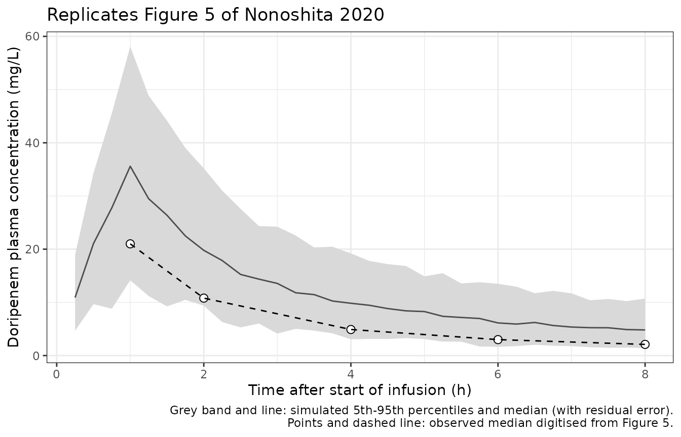
vpc_cmp <- vpc_sum |>
  dplyr::inner_join(fig5_obs_median, by = "time") |>
  dplyr::mutate(ratio = p50 / obs_median)
stopifnot(nrow(vpc_cmp) == 5L)

vpc_cmp |>
  dplyr::select(time, obs_median, p50, ratio) |>
  dplyr::rename(
    "Time (h)" = time,
    "Figure 5 observed median (mg/L)" = obs_median,
    "Simulated median (mg/L)" = p50,
    "Simulated / observed" = ratio
  ) |>
knitr::kable(digits = 2)| Time (h) | Figure 5 observed median (mg/L) | Simulated median (mg/L) | Simulated / observed |
|---|---|---|---|
| 1 | 21.0 | 35.58 | 1.69 |
| 2 | 10.8 | 19.78 | 1.83 |
| 4 | 4.9 | 9.83 | 2.01 |
| 6 | 3.0 | 6.14 | 2.05 |
| 8 | 2.1 | 4.82 | 2.29 |
The simulated median sits about 1.7-2.3-fold above the observed median at every sampling time. This is not a property of the virtual cohort: the typical non-CRRT subject alone (V1 = 10.04 L, CL = 3.65 L/h) reaches 36.4 mg/L at the end of the 500 mg infusion, while the paper’s own population predictions (Figure 4, upper left) do not exceed about 30 mg/L and cluster around 20 mg/L at 1 h. The reasons are set out under “Assumptions and deviations”; the parameters have not been adjusted.
# The discrepancy is structural (every time point, same direction), so the
# centre of the ratios is a stable property of the printed parameters. A
# change to any transcribed clearance or volume moves it by tens of percent.
stopifnot(
  stats::median(vpc_cmp$ratio) > 1.4,
  stats::median(vpc_cmp$ratio) < 3.0
)
Non-compartmental analysis
The paper reports no NCA. PKNCA is used here as an internal
consistency check: after a single dose, Dose / AUC0-inf
must return each subject’s total clearance. The simulation uses the
individual predictions (no residual error) out to 48 h so that the
extrapolated fraction of AUC is small.
ev_nca <- rxode2::et(amt = 500, dur = 1, cmt = "central") |>
  rxode2::et(c(seq(0, 2, by = 0.1), seq(2.25, 12, by = 0.25), seq(12.5, 48, by = 0.5)), cmt = "central") |>
  rxode2::et(id = cohort$id) |>
  as.data.frame() |>
  dplyr::left_join(cohort, by = "id")

sim_nca <- rxode2::rxSolve(
  mod, events = ev_nca, returnType = "data.frame", keep = "arm",
  rtol = 1e-10, atol = 1e-12
)
stopifnot(all(sim_nca$Cc >= -1e-6 * max(sim_nca$Cc, na.rm = TRUE), na.rm = TRUE))

conc_df <- sim_nca |>
  dplyr::filter(!is.na(Cc)) |>
  dplyr::mutate(Cc = pmax(Cc, 0), treatment = arm) |>
  dplyr::select(id, time, Cc, treatment)

dose_df <- cohort |>
  dplyr::transmute(id, time = 0, amt = 500, treatment = arm)

conc_obj <- PKNCA::PKNCAconc(conc_df, Cc ~ time | treatment + id, concu = "mg/L", timeu = "h")
dose_obj <- PKNCA::PKNCAdose(dose_df, amt ~ time | treatment + id, doseu = "mg", route = "intravascular", duration = 1)
intervals <- data.frame(
  start = 0, end = Inf,
  cmax = TRUE, tmax = TRUE, aucinf.obs = TRUE, half.life = TRUE, cl.obs = TRUE
)
nca_res <- PKNCA::pk.nca(PKNCA::PKNCAdata(conc_obj, dose_obj, intervals = intervals))

nca_df <- as.data.frame(nca_res)
summary(nca_res)
#>  Interval Start Interval End treatment   N Cmax (mg/L)          Tmax (h)
#>               0          Inf      CRRT 150 36.0 [10.2] 1.00 [1.00, 1.00]
#>               0          Inf   No CRRT 200 36.1 [11.1] 1.00 [1.00, 1.00]
#>  Half-life (h) AUCinf,obs (h*mg/L) CL (based on AUCinf,obs) (mg/(h*mg/L))
#>    4.53 [1.05]          138 [19.9]                            3.62 [19.9]
#>    4.51 [1.27]          133 [27.7]                            3.75 [27.7]
#>
#> Caption: Cmax, AUCinf,obs, CL (based on AUCinf,obs): geometric mean and geometric coefficient of variation; Tmax: median and range; Half-life: arithmetic mean and standard deviation; N: number of subjects
cl_nca <- nca_df |>
  dplyr::filter(PPTESTCD == "cl.obs") |>
  dplyr::select(id, treatment, cl_nca = PPORRES)
cl_ind <- sim_nca |>
  dplyr::filter(time == 1) |>
  dplyr::select(id, cl)
cl_chk <- dplyr::inner_join(cl_nca, cl_ind, by = "id") |>
  dplyr::mutate(pct_diff = 100 * (cl_nca / cl - 1))
stopifnot(nrow(cl_chk) == N_OFF + N_ON)

cl_chk |>
  dplyr::group_by(treatment) |>
  dplyr::summarise(
    median_cl_model = stats::median(cl),
    median_cl_nca = stats::median(cl_nca),
    median_pct_diff = stats::median(pct_diff),
    .groups = "drop"
  ) |>
  dplyr::rename(
    "Arm" = treatment,
    "Median model CL (L/h)" = median_cl_model,
    "Median NCA Dose/AUCinf (L/h)" = median_cl_nca,
    "Median difference (%)" = median_pct_diff
  ) |>
knitr::kable(digits = 2)| Arm | Median model CL (L/h) | Median NCA Dose/AUCinf (L/h) | Median difference (%) |
|---|---|---|---|
| CRRT | 3.63 | 3.63 | 0 |
| No CRRT | 3.74 | 3.74 | 0 |
Probability of target attainment (Table 4)
Table 4 gives the probability of attaining 40% and 100% of the dosing interval with free doripenem above an MIC of 2 mg/L (and 100% above 4 x MIC) at steady state, for 1 h intermittent infusion (InI) and 4 h extended infusion (ExI) every 8 h, and for continuous infusion (CI) of the same daily dose. Free concentration is total concentration times the 0.919 unbound fraction.
The Methods do not state the virtual-cohort sizes, the creatinine-clearance distribution within each band, the filtrate flow used for CRRT subjects, or whether residual error was added. This replication draws creatinine clearance uniformly within each band (the 0-30 band from 10 mL/min), uses a filtrate flow of 1.2 L/h (the middle of the reported range) and simulates without residual error, 200 subjects per arm.
rxode2::rxSetSeed(20201219)
set.seed(20201219)
N_PTA <- 200L
MIC <- 2
FU <- 0.919

bands <- tibble::tribble(
  ~band,          ~lo, ~hi, ~crrt,
  "0 < Ccr <= 30",  10,  30,     1,
  "0 < Ccr <= 30",  10,  30,     0,
  "30 < Ccr <= 60", 30,  60,     1,
  "30 < Ccr <= 60", 30,  60,     0,
  "60 < Ccr <= 90", 60,  90,     0
)
pta_arms <- tidyr::expand_grid(bands, method = c("InI", "ExI"), dose = c(250, 500, 1000, 2000)) |>
  dplyr::mutate(arm_id = dplyr::row_number())

make_pta_arm <- function(a) {
  ids <- (a$arm_id - 1L) * N_PTA + seq_len(N_PTA)
  covs <- tibble::tibble(
    id = ids,
    CRCL = stats::runif(N_PTA, a$lo, a$hi),
    RRT_CRRT_STATUS = a$crrt,
    RRT_CRRT_EFFLUENT_FLOW = 1200 * a$crrt,
    arm_id = a$arm_id
  )
  rxode2::et(amt = a$dose, dur = if (a$method == "InI") 1 else 4, ii = 8, ss = 1, cmt = "central") |>
    rxode2::et(round(seq(0, 8, by = 0.1), 6), cmt = "central") |>
    rxode2::et(id = ids) |>
    as.data.frame() |>
    dplyr::left_join(covs, by = "id")
}
ev_pta <- dplyr::bind_rows(lapply(split(pta_arms, pta_arms$arm_id), make_pta_arm))

sim_pta <- rxode2::rxSolve(
  mod, events = ev_pta, returnType = "data.frame", keep = "arm_id",
  maxsteps = 1e6
)

pta_sim <- sim_pta |>
  dplyr::filter(time > 0) |>
  dplyr::group_by(arm_id, id) |>
  dplyr::summarise(
    ft_mic = mean(FU * Cc > MIC),
    ft_mic4 = mean(FU * Cc > 4 * MIC),
    .groups = "drop"
  ) |>
  dplyr::group_by(arm_id) |>
  dplyr::summarise(
    pta40 = 100 * mean(ft_mic >= 0.4),
    pta100 = 100 * mean(ft_mic >= 1),
    pta100x4 = 100 * mean(ft_mic4 >= 1),
    .groups = "drop"
  ) |>
  dplyr::left_join(pta_arms, by = "arm_id")

# Published Table 4, InI and ExI rows (40% fT>MIC, 100% fT>MIC, 100% fT>MICx4).
table4 <- tibble::tribble(
  ~band,            ~crrt, ~method, ~dose, ~pub40, ~pub100, ~pub100x4,
  "0 < Ccr <= 30",      1, "InI",   2000,   99.7,    86.6,     81.5,
  "0 < Ccr <= 30",      1, "InI",   1000,   99.5,    81.5,     61.6,
  "0 < Ccr <= 30",      1, "InI",    500,   99.0,    73.7,     39.9,
  "0 < Ccr <= 30",      1, "InI",    250,   98.2,    61.6,     12.2,
  "0 < Ccr <= 30",      0, "InI",   2000,  100.0,    97.5,     94.5,
  "0 < Ccr <= 30",      0, "InI",   1000,  100.0,    96.4,     91.0,
  "0 < Ccr <= 30",      0, "InI",    500,  100.0,    94.5,     82.8,
  "0 < Ccr <= 30",      0, "InI",    250,   99.0,    91.0,     66.7,
  "0 < Ccr <= 30",      1, "ExI",   2000,  100.0,   100.0,    100.0,
  "0 < Ccr <= 30",      1, "ExI",   1000,  100.0,   100.0,     99.4,
  "0 < Ccr <= 30",      1, "ExI",    500,  100.0,   100.0,     94.3,
  "0 < Ccr <= 30",      1, "ExI",    250,  100.0,    99.4,     58.8,
  "0 < Ccr <= 30",      0, "ExI",   2000,  100.0,   100.0,    100.0,
  "0 < Ccr <= 30",      0, "ExI",   1000,  100.0,   100.0,    100.0,
  "0 < Ccr <= 30",      0, "ExI",    500,  100.0,   100.0,     99.8,
  "0 < Ccr <= 30",      0, "ExI",    250,  100.0,   100.0,     91.4,
  "30 < Ccr <= 60",     1, "InI",   2000,   98.9,    74.8,     58.8,
  "30 < Ccr <= 60",     1, "InI",   1000,   98.5,    68.5,     44.4,
  "30 < Ccr <= 60",     1, "InI",    500,   97.8,    58.8,     24.1,
  "30 < Ccr <= 60",     1, "InI",    250,   95.8,    44.4,      5.1,
  "30 < Ccr <= 60",     0, "InI",   2000,   99.8,    87.3,     75.9,
  "30 < Ccr <= 60",     0, "InI",   1000,   99.6,    82.9,     63.9,
  "30 < Ccr <= 60",     0, "InI",    500,   99.4,    75.9,     44.3,
  "30 < Ccr <= 60",     0, "InI",    250,   99.0,    63.9,     20.6,
  "30 < Ccr <= 60",     1, "ExI",   2000,  100.0,   100.0,     99.8,
  "30 < Ccr <= 60",     1, "ExI",   1000,  100.0,   100.0,     98.4,
  "30 < Ccr <= 60",     1, "ExI",    500,  100.0,    99.8,     85.1,
  "30 < Ccr <= 60",     1, "ExI",    250,   99.8,    98.4,     35.1,
  "30 < Ccr <= 60",     0, "ExI",   2000,  100.0,   100.0,    100.0,
  "30 < Ccr <= 60",     0, "ExI",   1000,  100.0,   100.0,     99.9,
  "30 < Ccr <= 60",     0, "ExI",    500,  100.0,   100.0,     92.5,
  "30 < Ccr <= 60",     0, "ExI",    250,  100.0,    99.9,     57.8,
  "60 < Ccr <= 90",     0, "InI",   2000,   99.4,    75.9,     59.4,
  "60 < Ccr <= 90",     0, "InI",   1000,   98.9,    69.3,     44.5,
  "60 < Ccr <= 90",     0, "InI",    500,   98.3,    59.4,     23.6,
  "60 < Ccr <= 90",     0, "InI",    250,   96.8,    44.5,      7.6,
  "60 < Ccr <= 90",     0, "ExI",   2000,  100.0,   100.0,    100.0,
  "60 < Ccr <= 90",     0, "ExI",   1000,  100.0,   100.0,     99.7,
  "60 < Ccr <= 90",     0, "ExI",    500,  100.0,   100.0,     86.4,
  "60 < Ccr <= 90",     0, "ExI",    250,  100.0,    99.7,     33.0
)

pta_cmp <- dplyr::inner_join(pta_sim, table4, by = c("band", "crrt", "method", "dose"))
stopifnot(nrow(pta_cmp) == nrow(table4), nrow(pta_cmp) == nrow(pta_arms))

pta_cmp |>
  dplyr::arrange(band, dplyr::desc(crrt), method, dplyr::desc(dose)) |>
  dplyr::mutate(crrt = ifelse(crrt == 1, "On", "Off")) |>
  dplyr::select(band, method, crrt, dose, pub40, pta40, pub100, pta100, pub100x4, pta100x4) |>
  dplyr::rename(
    "Renal function" = band,
    "Infusion" = method,
    "CRRT" = crrt,
    "Dose (mg)" = dose,
    "40% fT>MIC, paper" = pub40,
    "40% fT>MIC, sim" = pta40,
    "100% fT>MIC, paper" = pub100,
    "100% fT>MIC, sim" = pta100,
    "100% fT>4xMIC, paper" = pub100x4,
    "100% fT>4xMIC, sim" = pta100x4
  ) |>
knitr::kable(digits = 1)| Renal function | Infusion | CRRT | Dose (mg) | 40% fT>MIC, paper | 40% fT>MIC, sim | 100% fT>MIC, paper | 100% fT>MIC, sim | 100% fT>4xMIC, paper | 100% fT>4xMIC, sim |
|---|---|---|---|---|---|---|---|---|---|
| 0 < Ccr <= 30 | ExI | On | 2000 | 100.0 | 100 | 100.0 | 100.0 | 100.0 | 100.0 |
| 0 < Ccr <= 30 | ExI | On | 1000 | 100.0 | 100 | 100.0 | 100.0 | 99.4 | 100.0 |
| 0 < Ccr <= 30 | ExI | On | 500 | 100.0 | 100 | 100.0 | 100.0 | 94.3 | 97.5 |
| 0 < Ccr <= 30 | ExI | On | 250 | 100.0 | 100 | 99.4 | 100.0 | 58.8 | 22.0 |
| 0 < Ccr <= 30 | InI | On | 2000 | 99.7 | 100 | 86.6 | 100.0 | 81.5 | 100.0 |
| 0 < Ccr <= 30 | InI | On | 1000 | 99.5 | 100 | 81.5 | 100.0 | 61.6 | 100.0 |
| 0 < Ccr <= 30 | InI | On | 500 | 99.0 | 100 | 73.7 | 100.0 | 39.9 | 86.0 |
| 0 < Ccr <= 30 | InI | On | 250 | 98.2 | 100 | 61.6 | 100.0 | 12.2 | 4.0 |
| 0 < Ccr <= 30 | ExI | Off | 2000 | 100.0 | 100 | 100.0 | 100.0 | 100.0 | 100.0 |
| 0 < Ccr <= 30 | ExI | Off | 1000 | 100.0 | 100 | 100.0 | 100.0 | 100.0 | 100.0 |
| 0 < Ccr <= 30 | ExI | Off | 500 | 100.0 | 100 | 100.0 | 100.0 | 99.8 | 100.0 |
| 0 < Ccr <= 30 | ExI | Off | 250 | 100.0 | 100 | 100.0 | 100.0 | 91.4 | 96.0 |
| 0 < Ccr <= 30 | InI | Off | 2000 | 100.0 | 100 | 97.5 | 100.0 | 94.5 | 100.0 |
| 0 < Ccr <= 30 | InI | Off | 1000 | 100.0 | 100 | 96.4 | 100.0 | 91.0 | 100.0 |
| 0 < Ccr <= 30 | InI | Off | 500 | 100.0 | 100 | 94.5 | 100.0 | 82.8 | 100.0 |
| 0 < Ccr <= 30 | InI | Off | 250 | 99.0 | 100 | 91.0 | 100.0 | 66.7 | 80.0 |
| 30 < Ccr <= 60 | ExI | On | 2000 | 100.0 | 100 | 100.0 | 100.0 | 99.8 | 100.0 |
| 30 < Ccr <= 60 | ExI | On | 1000 | 100.0 | 100 | 100.0 | 100.0 | 98.4 | 100.0 |
| 30 < Ccr <= 60 | ExI | On | 500 | 100.0 | 100 | 99.8 | 100.0 | 85.1 | 71.5 |
| 30 < Ccr <= 60 | ExI | On | 250 | 99.8 | 100 | 98.4 | 99.0 | 35.1 | 0.5 |
| 30 < Ccr <= 60 | InI | On | 2000 | 98.9 | 100 | 74.8 | 100.0 | 58.8 | 100.0 |
| 30 < Ccr <= 60 | InI | On | 1000 | 98.5 | 100 | 68.5 | 100.0 | 44.4 | 95.5 |
| 30 < Ccr <= 60 | InI | On | 500 | 97.8 | 100 | 58.8 | 100.0 | 24.1 | 32.0 |
| 30 < Ccr <= 60 | InI | On | 250 | 95.8 | 100 | 44.4 | 96.5 | 5.1 | 0.0 |
| 30 < Ccr <= 60 | ExI | Off | 2000 | 100.0 | 100 | 100.0 | 100.0 | 100.0 | 100.0 |
| 30 < Ccr <= 60 | ExI | Off | 1000 | 100.0 | 100 | 100.0 | 100.0 | 99.9 | 100.0 |
| 30 < Ccr <= 60 | ExI | Off | 500 | 100.0 | 100 | 100.0 | 100.0 | 92.5 | 95.5 |
| 30 < Ccr <= 60 | ExI | Off | 250 | 100.0 | 100 | 99.9 | 100.0 | 57.8 | 9.0 |
| 30 < Ccr <= 60 | InI | Off | 2000 | 99.8 | 100 | 87.3 | 100.0 | 75.9 | 100.0 |
| 30 < Ccr <= 60 | InI | Off | 1000 | 99.6 | 100 | 82.9 | 100.0 | 63.9 | 100.0 |
| 30 < Ccr <= 60 | InI | Off | 500 | 99.4 | 100 | 75.9 | 100.0 | 44.3 | 71.0 |
| 30 < Ccr <= 60 | InI | Off | 250 | 99.0 | 100 | 63.9 | 100.0 | 20.6 | 0.0 |
| 60 < Ccr <= 90 | ExI | Off | 2000 | 100.0 | 100 | 100.0 | 100.0 | 100.0 | 100.0 |
| 60 < Ccr <= 90 | ExI | Off | 1000 | 100.0 | 100 | 100.0 | 100.0 | 99.7 | 99.5 |
| 60 < Ccr <= 90 | ExI | Off | 500 | 100.0 | 100 | 100.0 | 100.0 | 86.4 | 19.5 |
| 60 < Ccr <= 90 | ExI | Off | 250 | 100.0 | 100 | 99.7 | 99.5 | 33.0 | 0.0 |
| 60 < Ccr <= 90 | InI | Off | 2000 | 99.4 | 100 | 75.9 | 100.0 | 59.4 | 100.0 |
| 60 < Ccr <= 90 | InI | Off | 1000 | 98.9 | 100 | 69.3 | 100.0 | 44.5 | 88.0 |
| 60 < Ccr <= 90 | InI | Off | 500 | 98.3 | 100 | 59.4 | 100.0 | 23.6 | 1.0 |
| 60 < Ccr <= 90 | InI | Off | 250 | 96.8 | 100 | 44.5 | 86.0 | 7.6 | 0.0 |
For continuous infusion the steady-state concentration is
Css = (daily dose / 24) / CL, so a subject attains 100% fT
> MIC exactly when 0.919 x Css > MIC. That needs only
each subject’s clearance.
cl_pta <- sim_pta |>
  dplyr::filter(time == 0) |>
  dplyr::distinct(id, arm_id, cl) |>
  dplyr::left_join(pta_arms, by = "arm_id") |>
  dplyr::filter(method == "InI") |>
  dplyr::mutate(daily_dose = 3 * dose)

pta_ci <- cl_pta |>
  dplyr::mutate(css_free = FU * daily_dose / 24 / cl) |>
  dplyr::group_by(band, crrt, daily_dose) |>
  dplyr::summarise(
    pta100 = 100 * mean(css_free > MIC),
    pta100x4 = 100 * mean(css_free > 4 * MIC),
    .groups = "drop"
  )

pta_ci |>
  dplyr::mutate(crrt = ifelse(crrt == 1, "On", "Off")) |>
  dplyr::arrange(band, dplyr::desc(crrt), dplyr::desc(daily_dose)) |>
  dplyr::rename(
    "Renal function" = band,
    "CRRT" = crrt,
    "Daily dose (mg)" = daily_dose,
    "100% fT>MIC, sim" = pta100,
    "100% fT>4xMIC, sim" = pta100x4
  ) |>
knitr::kable(digits = 1)| Renal function | CRRT | Daily dose (mg) | 100% fT>MIC, sim | 100% fT>4xMIC, sim |
|---|---|---|---|---|
| 0 < Ccr <= 30 | On | 6000 | 100 | 100.0 |
| 0 < Ccr <= 30 | On | 3000 | 100 | 100.0 |
| 0 < Ccr <= 30 | On | 1500 | 100 | 100.0 |
| 0 < Ccr <= 30 | On | 750 | 100 | 97.0 |
| 0 < Ccr <= 30 | Off | 6000 | 100 | 100.0 |
| 0 < Ccr <= 30 | Off | 3000 | 100 | 100.0 |
| 0 < Ccr <= 30 | Off | 1500 | 100 | 100.0 |
| 0 < Ccr <= 30 | Off | 750 | 100 | 100.0 |
| 30 < Ccr <= 60 | On | 6000 | 100 | 100.0 |
| 30 < Ccr <= 60 | On | 3000 | 100 | 100.0 |
| 30 < Ccr <= 60 | On | 1500 | 100 | 100.0 |
| 30 < Ccr <= 60 | On | 750 | 100 | 64.0 |
| 30 < Ccr <= 60 | Off | 6000 | 100 | 100.0 |
| 30 < Ccr <= 60 | Off | 3000 | 100 | 100.0 |
| 30 < Ccr <= 60 | Off | 1500 | 100 | 100.0 |
| 30 < Ccr <= 60 | Off | 750 | 100 | 96.0 |
| 60 < Ccr <= 90 | Off | 6000 | 100 | 100.0 |
| 60 < Ccr <= 90 | Off | 3000 | 100 | 100.0 |
| 60 < Ccr <= 90 | Off | 1500 | 100 | 100.0 |
| 60 < Ccr <= 90 | Off | 750 | 100 | 12.5 |
The paper’s qualitative conclusions are reproduced: every InI and ExI regimen reaches over 90% PTA for 40% fT > MIC, and every continuous-infusion dose reaches over 90% PTA for 100% fT > MIC in every renal-function and CRRT condition. The stricter 100% targets do not match cell by cell. Table 4 changes little with dose (for example 44.5% at 250 mg and 75.9% at 2000 mg for 100% fT > MIC with InI at 60 < Ccr <= 90), whereas the simulation moves from near 0% to 100% across the same doses: it is higher than Table 4 at the upper doses and, for 100% fT > 4 x MIC, lower at the lowest ones. An eight-fold dose increase moving PTA as little as Table 4 shows requires far more between-subject spread than the printed 7-24% IIV provides, which suggests residual error was added to the simulated concentrations. With the printed clearances also giving about twice the exposure of the paper’s own fit (see the VPC above), the stricter-target cells are not expected to match.
stopifnot(
  # Table 4 / Results: 'For the target of 40% fT > MIC, all three infusion
  # methods of all dosages achieved over 90% PTA regardless of renal function
  # and CRRT.' The simulated cells sit at or near 100%, far from the bound.
  all(pta_cmp$pta40 > 90),
  # Results: 'When administered by CI, all dosages (750-6000 mg) achieved
  # over 90% PTA for 100% fT > MIC'.
  nrow(pta_ci) == 20L,
  all(pta_ci$pta100 > 90)
)
Assumptions and deviations
-
The printed parameters do not reproduce the paper’s own
fit. Transcribed as printed, the model predicts about twice the
concentrations of the paper’s Figure 5 observed medians and Figure 4
population predictions after the 500 mg dose that 20 of the 21 patients
received. Mass balance on the Figure 5 median profile (AUC0-inf of
roughly 65-70 mg.h/L) implies a pooled clearance near 7.4 L/h rather
than the 3.65 and 3.81 L/h the paper reports. An earlier paper from the
same unit (Tanaka et al., Biol Pharm Bull 2017;40:1226-1231, doi:10.1248/bpb.b17-00008) studied 12 non-CRRT ICU
patients whose creatinine clearance summary (mean 76.0 mL/min, range
20.7-155.6) matches the non-CRRT stratum here, and reported Bayesian
individual clearances of 9.0 +/- 3.1 L/h, again far above 3.65 L/h. A
dose recorded at half its true amount in the estimation dataset would
halve every clearance and volume and would explain the figures, but the
paper gives no basis for that correction, so the parameters are left
exactly as printed. For clinical or exposure work, treat the absolute
clearance and volume values with caution; the covariate structure
(stratum-specific creatinine-clearance effects and the additive
QE x 0.919CRRT arm) is unaffected by this issue. -
IIV order for the two body clearances. The Results
sentence lists the inter-individual variability of
CLbody(CRRT)andCLbody(non-CRRT)as 7.3% and 22.2% in that order, while Table 3 assigns 7.3% to the non-CRRT and 22.2% to the CRRT stratum. The Discussion (“non-CRRT group: 17.0-7.3%, CRRT group: 29.4-22.2%”) agrees with Table 3, which is used here. The shrinkage values in the same Results sentence are therefore probably in the same swapped order. - Residual error. The Methods state an additive error model. Table 3 prints the final residual row as an estimate of 0.70 (row unit ug/mL) together with a percentage of 36.5%, and the Results call 36.5% the residual variability; the base-model row (0.016 with 42.3%) and the bootstrap median (0.02) do not resolve which is the fitted scale. Both numbers are encoded, as an additive SD of 0.70 mg/L plus a proportional SD of 0.365. The widening of the Figure 5 prediction interval at the 1 h peak supports a concentration-proportional component, and its 5th percentile falling below zero at 6-8 h supports an additive one. Residual error does not affect the typical-value, NCA or PTA sections above.
-
CRRT inputs. CRRT status is treated as fixed per
subject over the 8 h sampling interval. The filtrate flow enters as
RRT_CRRT_EFFLUENT_FLOWin mL/h (the paper’s QE in L/h times 1000); the paper’s QE range (0.6-1.8 L/h) equals the sum of its dialysate and replacement-fluid ranges. The 0.919 sieving coefficient is the literature unbound fraction and was not estimated. Per-patient filtrate flows are not published, so the virtual cohort draws them uniformly over the reported range. - Creatinine clearance is raw Cockcroft-Gault in mL/min (not BSA-normalized). In CRRT patients serum creatinine is also cleared by the circuit, so the value reflects combined kidney-plus-circuit function; the model uses the CRRT-stratum exponent and median for these patients, as the paper does.
- Screened but not retained: body weight (on CL_body, V1, V2) and serum albumin (on V1, V2 and CL_CRRT). Body weight on V1 and albumin on CL_CRRT entered the full model and were removed in backward elimination (Table 2).
- Virtual cohort. Creatinine clearance is drawn from a log-normal distribution parameterised with the Table 1 stratum mean and SD and truncated to the observed range; for the PTA section it is drawn uniformly within each band (the lowest band from 10 mL/min) with a filtrate flow of 1.2 L/h, since the paper does not report its simulation settings.