Hwang_2022_tremelimumab • nlmixr2lib

Model and source

Citation: Hwang M, Chia YL, Zheng Y, Chen CC-K, He J, Song X, Zhou D, Goldberg SB, Siu LL, Planchard D, Peters S, Mann H, Krug L, Even C. Population pharmacokinetic modelling of tremelimumab in patients with advanced solid tumours and the impact of disease status on time-varying clearance. Br J Clin Pharmacol. 2023;89(5):1601-1616. doi:[10.1111/bcp.15622](https://doi.org/10.1111/bcp.15622)
Description: Two-compartment population PK model for tremelimumab (anti-CTLA-4 IgG2 kappa) with regimen-dependent sigmoidal time-varying clearance in adults with advanced solid tumours, dosed as monotherapy or in combination with durvalumab.
Modality: Therapeutic monoclonal antibody (IgG2 kappa), IV infusion.

Tremelimumab is a fully human anti-CTLA-4 IgG2 kappa monoclonal antibody. Hwang 2022 pooled PK data from five Phase 1 / 2 studies (956 patients, 4,043 PK records after exclusions) and externally validated against four additional Phase 2 / 3 studies (554 patients). The final model is a linear two-compartment IV model with first-order elimination and a sigmoidal time-varying clearance term whose direction depends on therapy regimen: clearance increases over time on monotherapy and decreases over time when tremelimumab is co-administered with durvalumab. Baseline body weight (power) and baseline serum albumin (power) are retained as continuous covariates on clearance, and body weight is also retained on central volume.

The structural model is:

$\mathrm{CL}_{i}(t) \;=\; 0.276\;\mathrm{L/day} \cdot \exp\!\left( \dfrac{(T_{\max,r} + \eta_{T_{\max},i})\, t^{\lambda_{r}}} {\mathrm{TC}_{50}^{\lambda_{r}} + t^{\lambda_{r}}} \right) \cdot \left(\dfrac{\mathrm{ALB}_{i}}{39}\right)^{-0.996} \cdot \left(\dfrac{\mathrm{WT}_{i}}{71}\right)^{0.638} \cdot \exp(\eta_{\mathrm{CL},i})$

$V_{c,i} \;=\; 3.64\;\mathrm{L} \cdot \left(\dfrac{\mathrm{WT}_{i}}{71}\right)^{0.606} \cdot \exp(\eta_{V_{c},i}), \qquad Q = 0.357\;\mathrm{L/day}, \qquad V_{p} = 2.40\;\mathrm{L}$

with regimen-specific $(T_{\max,\,\mathrm{mono}}, \lambda_{\mathrm{mono}}) = (0.151, 14.5)$ and $(T_{\max,\,\mathrm{combo}}, \lambda_{\mathrm{combo}}) = (-0.187, 3.20)$ and a common $\mathrm{TC}_{50} = 95.1\;\mathrm{days}$ (Hwang 2022 Table 3 and the final-model equations on page 1609).

Population

The final-model population comprised 956 patients (development dataset; Table 2) pooled from five trials:

Study 02 (NCT01938612, n = 122 enrolled / 110 included): combination with durvalumab in biliary tract cancer, oesophageal cancer, and squamous cell carcinoma of the head and neck.
Study 06 (NCT02000947, n = 351 / 197): combination with durvalumab in non-small-cell lung cancer.
Study 10 (NCT02261220, n = 372 / 279): combination with durvalumab in urothelial cancer and other solid tumours.
DETERMINE (NCT01843374, n = 374 / 326): tremelimumab monotherapy in pleural / peritoneal malignant mesothelioma.
D4884C00001 (NCT02527434, n = 61 / 46): tremelimumab monotherapy (750 mg flat) or combination with durvalumab (75 mg flat) in urothelial, triple-negative breast, and pancreatic ductal cancers.

Baseline demographics (Hwang 2022 Table 2):

Age 65 (range 22-87) years; weight 71.6 (35.5-149.0) kg; BMI 25.2 (13.8-50.9).
Sex: 63.2% male, 36.8% female.
Race: 75.5% White, 19.3% Asian, 1.4% Black, 3.9% Other.
Country: Japan 6.7%, Korea 7.7%, Other 85.6%.
Treatment: tremelimumab monotherapy 38.8%, in combination with durvalumab 61.2%.
ECOG performance status: 0 = 38.9%, 1 = 60.9%, 2 = 0.1%.
Median tumour size 73 mm (10-668); median baseline serum albumin 39 g/L (15-52); median baseline LDH 209.5 U/L.
Postbaseline ADA-positive: 6.1% overall (2.8% on monotherapy, 7.8% on combination).

External validation (n = 554) used four phase 2 / 3 studies (ARCTIC, EAGLE, CONDOR, MYSTIC) and is not part of the parameter estimation; this vignette therefore simulates only the development-dataset regimens.

The same metadata is available programmatically via readModelDb("Hwang_2022_tremelimumab")$population.

Source trace

The per-parameter origin is recorded as an in-file comment next to each ini() entry in inst/modeldb/specificDrugs/Hwang_2022_tremelimumab.R. The table below collects them in one place for review.

Parameter (model name)	Value	Source
`lcl` (CL_BASE, L/day)	log(0.276)	Hwang 2022 Table 3, CL = 0.276 L/day
`lvc` (Vc, L)	log(3.64)	Hwang 2022 Table 3, Vc = 3.64 L
`lq` (Q, L/day)	log(0.357)	Hwang 2022 Table 3, Q = 0.357 L/day
`lvp` (Vp, L)	log(2.40)	Hwang 2022 Table 3, Vp = 2.40 L
`e_alb_cl` (power, ALB on CL)	-0.996	Hwang 2022 Table 3, covariate 1 ALB on CL
`e_wt_vc` (power, WT on Vc)	0.606	Hwang 2022 Table 3, covariate 2 WT on Vc
`e_wt_cl` (power, WT on CL)	0.638	Hwang 2022 Table 3, covariate 3 WT on CL
`cl_tmax_mono` (Tmax mono)	0.151	Hwang 2022 Table 3, covariate 4 Tmax (monotherapy)
`cl_tc50` (TC50, days)	95.1	Hwang 2022 Table 3, covariate 5 TC50 (common)
`cl_lambda_mono` (lambda mono)	14.5	Hwang 2022 Table 3, covariate 6 Lambda (monotherapy)
`cl_tmax_combo` (Tmax combo)	-0.187	Hwang 2022 Table 3, covariate 7 Tmax (combination therapy)
`cl_lambda_combo` (lambda combo)	3.20	Hwang 2022 Table 3, covariate 8 Lambda (combination)
`etalcl` (omega^2 on lcl)	0.113 (33.6% CV)	Hwang 2022 Table 3, IIV on CL
`etalvc` (omega^2 on lvc)	0.0536 (23.2% CV)	Hwang 2022 Table 3, IIV on Vc
`etacl_tmax` (omega^2 on Tmax)	0.151 (38.9% CV)	Hwang 2022 Table 3, IIV on Tmax
`propSd`	0.306	Hwang 2022 Table 3, proportional residual error
`addSd`	0.119 ug/mL	Hwang 2022 Table 3, additive residual error

Equations: structural two-compartment micro-constant form (NM-TRAN ADVAN6); the full final-model equations for CL_i and Vc_i are reproduced verbatim from page 1609 of Hwang 2022, with the time-varying multiplier EMPIR = (Tmax + ETA) * TIME^lambda / (TC50^lambda + TIME^lambda) taken from the supplement’s NONMEM control stream (Supplementary Results).

Reference covariates (Hwang 2022 page 1609 final-model equations): WT = 71 kg, ALB = 39 g/L. The two regimen-specific (Tmax, lambda) estimates share a common TC50.

Errata

No published errata or corrigenda were located for Hwang 2022 (PubMed search, Crossref relations, OpenAlex retraction status; query as of 2026-04-27). One minor narrative-vs-table discrepancy is noted below under Assumptions and deviations: the paper’s prose on page 1609 cites Tmax = 0.157 for the monotherapy regimen, while Table 3 reports 0.151 ± 0.00405. The Table 3 value is used here per the skill’s preference for results-table point estimates over narrative summaries.

Virtual cohort

Original observed PK data are not publicly available. The simulations below use a virtual cohort whose demographics approximate the pooled Hwang 2022 development population (Table 2). Continuous covariates are drawn from log-normal / normal shapes anchored to the reported median and range; binary / categorical covariates match the reported marginal distributions.

set.seed(2022)
n_subj <- 200

cohort <- tibble::tibble(
  id          = seq_len(n_subj),
  WT          = pmin(pmax(rlnorm(n_subj, log(71.6), 0.22), 35.5), 149.0),
  ALB         = pmin(pmax(rnorm(n_subj, mean = 39, sd = 5), 15), 52),
  COMBO_DURVA = rbinom(n_subj, 1, 0.612)
)
summary(cohort[, c("WT", "ALB", "COMBO_DURVA")])
#>        WT              ALB         COMBO_DURVA  
#>  Min.   : 37.82   Min.   :26.73   Min.   :0.00  
#>  1st Qu.: 59.51   1st Qu.:35.37   1st Qu.:0.00  
#>  Median : 72.33   Median :38.44   Median :1.00  
#>  Mean   : 72.94   Mean   :38.70   Mean   :0.61  
#>  3rd Qu.: 84.35   3rd Qu.:41.75   3rd Qu.:1.00  
#>  Max.   :135.14   Max.   :52.00   Max.   :1.00

Two reference dosing regimens (the predominant regimens in the Hwang 2022 development dataset, Table 1) are simulated:

1 mg/kg Q4W in combination with durvalumab for 4 doses (the combination regimen used in Studies 02, 06, 10, ARCTIC, EAGLE, MYSTIC, and CONDOR).
10 mg/kg Q4W as monotherapy for 7 doses (the monotherapy regimen used in DETERMINE, ARCTIC, and CONDOR).

make_events <- function(pop, regimen) {
  if (regimen == "1 mg/kg + durva") {
    pop$COMBO_DURVA <- 1L
    dose_times <- seq(0, by = 28, length.out = 4)
    mg_per_kg  <- 1
  } else if (regimen == "10 mg/kg mono") {
    pop$COMBO_DURVA <- 0L
    dose_times <- seq(0, by = 28, length.out = 7)
    mg_per_kg  <- 10
  } else stop("unknown regimen")

  amt_per_subj <- pop$WT * mg_per_kg
  d_dose <- pop |>
    mutate(AMT = amt_per_subj) |>
    tidyr::crossing(TIME = dose_times) |>
    mutate(EVID = 1L, CMT = "central", DUR = 1 / 24, DV = NA_real_,
           treatment = regimen)
  d_obs <- pop |>
    tidyr::crossing(TIME = sort(unique(c(dose_times,
                                         seq(0, 365, by = 3))))) |>
    mutate(AMT = NA_real_, EVID = 0L, CMT = "central", DUR = NA_real_,
           DV = NA_real_, treatment = regimen)
  dplyr::bind_rows(d_dose, d_obs) |>
    dplyr::arrange(id, TIME, dplyr::desc(EVID)) |>
    as.data.frame()
}

events_combo <- make_events(cohort, "1 mg/kg + durva")
events_mono  <- make_events(cohort, "10 mg/kg mono")

Simulation

mod <- readModelDb("Hwang_2022_tremelimumab")

sim_combo <- rxode2::rxSolve(mod, events = events_combo,
                             returnType = "data.frame")
#> ℹ parameter labels from comments will be replaced by 'label()'
sim_mono  <- rxode2::rxSolve(mod, events = events_mono,
                             returnType = "data.frame")
#> ℹ parameter labels from comments will be replaced by 'label()'

sim <- dplyr::bind_rows(
  dplyr::mutate(sim_combo, treatment = "1 mg/kg + durva"),
  dplyr::mutate(sim_mono,  treatment = "10 mg/kg mono")
)

Concentration-time profiles (replicates Figure 3)

Hwang 2022 Figure 3 shows model-based simulations stratified by regimen: panel A is the 1 mg/kg combination arm and panel B is the 10 mg/kg monotherapy arm, each with the 95% prediction interval. The plot below reproduces the median and 5-95% prediction interval from the packaged model.

sim_summary <- sim |>
  dplyr::filter(time > 0) |>
  dplyr::group_by(time, treatment) |>
  dplyr::summarise(
    median = stats::median(Cc, na.rm = TRUE),
    lo     = stats::quantile(Cc, 0.05, na.rm = TRUE),
    hi     = stats::quantile(Cc, 0.95, na.rm = TRUE),
    .groups = "drop"
  )

ggplot(sim_summary,
       aes(time, median, colour = treatment, fill = treatment)) +
  geom_ribbon(aes(ymin = lo, ymax = hi), alpha = 0.15, colour = NA) +
  geom_line(linewidth = 1) +
  scale_y_log10() +
  labs(
    x = "Time since first dose (days)",
    y = "Tremelimumab concentration (ug/mL, log scale)",
    title = "Simulated tremelimumab PK by regimen",
    subtitle = paste0("Median and 90% prediction interval (N = ",
                      n_subj, " virtual patients per arm). ",
                      "Replicates Figure 3 of Hwang 2022."),
    caption = "Model: Hwang 2022 Br J Clin Pharmacol 89(5):1601-1616"
  ) +
  theme_bw()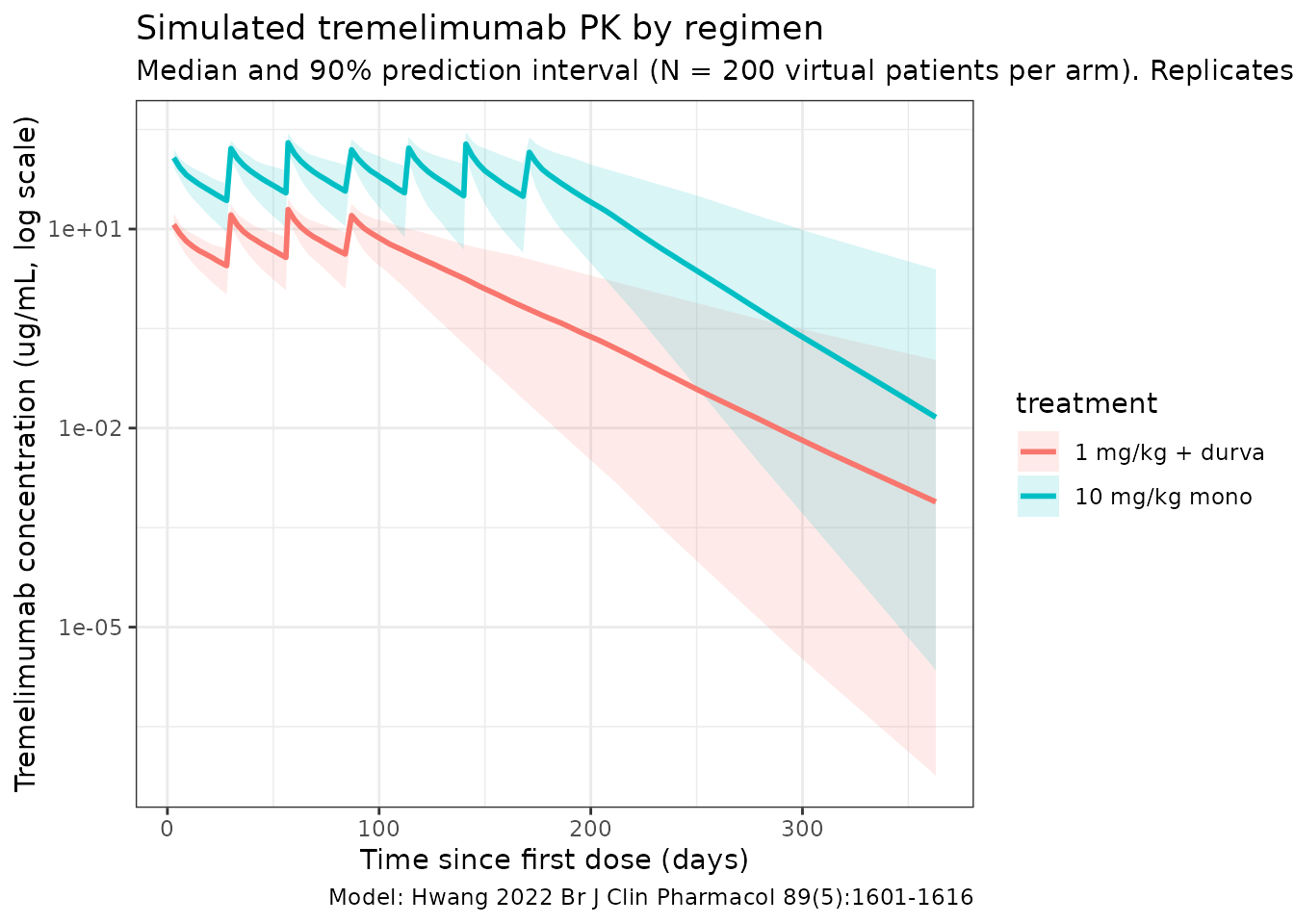

Time-varying clearance (replicates Figure 5 trends)

Hwang 2022 reports that, over one year of dosing, typical-value CL increases by ~16% on monotherapy and decreases by ~17% on the combination arm (page 1609, Discussion of the time-varying CL). The typical-value CL(t) / CL(0) curves below reproduce these trends at a reference subject (WT = 71 kg, ALB = 39 g/L, etas = 0).

typ_grid <- seq(0, 365, by = 5)

build_typ_events <- function(combo) {
  data.frame(
    id          = 1L,
    WT          = 71,
    ALB         = 39,
    COMBO_DURVA = combo,
    TIME        = c(0, typ_grid),
    AMT         = c(71, rep(NA_real_, length(typ_grid))),
    EVID        = c(1L, rep(0L, length(typ_grid))),
    CMT         = "central",
    DUR         = c(1 / 24, rep(NA_real_, length(typ_grid))),
    DV          = NA_real_
  )
}

mod_typ  <- rxode2::zeroRe(mod)
#> ℹ parameter labels from comments will be replaced by 'label()'
sim_typ_mono  <- rxode2::rxSolve(mod_typ, events = build_typ_events(0),
                                 returnType = "data.frame")
#> ℹ omega/sigma items treated as zero: 'etalcl', 'etalvc', 'etacl_tmax'
sim_typ_combo <- rxode2::rxSolve(mod_typ, events = build_typ_events(1),
                                 returnType = "data.frame")
#> ℹ omega/sigma items treated as zero: 'etalcl', 'etalvc', 'etacl_tmax'

cl_curves <- dplyr::bind_rows(
  dplyr::mutate(sim_typ_mono,  regimen = "Monotherapy"),
  dplyr::mutate(sim_typ_combo, regimen = "Combination with durvalumab")
) |>
  dplyr::filter(time > 0) |>
  dplyr::group_by(regimen) |>
  dplyr::mutate(cl_ratio = cl / cl[1]) |>
  dplyr::ungroup()

ggplot(cl_curves, aes(time, cl_ratio, colour = regimen)) +
  geom_hline(yintercept = 1, linetype = "dashed", colour = "grey40") +
  geom_line(linewidth = 1) +
  labs(
    x = "Time since first dose (days)",
    y = "CL(t) / CL(0)",
    title = "Time-varying clearance in Hwang 2022",
    subtitle = paste0("Typical reference subject (WT = 71 kg, ALB = 39 g/L). ",
                      "Asymptotes: monotherapy exp(0.151) = 1.163 (+16.3%); ",
                      "combination exp(-0.187) = 0.829 (-17.1%).")
  ) +
  theme_bw()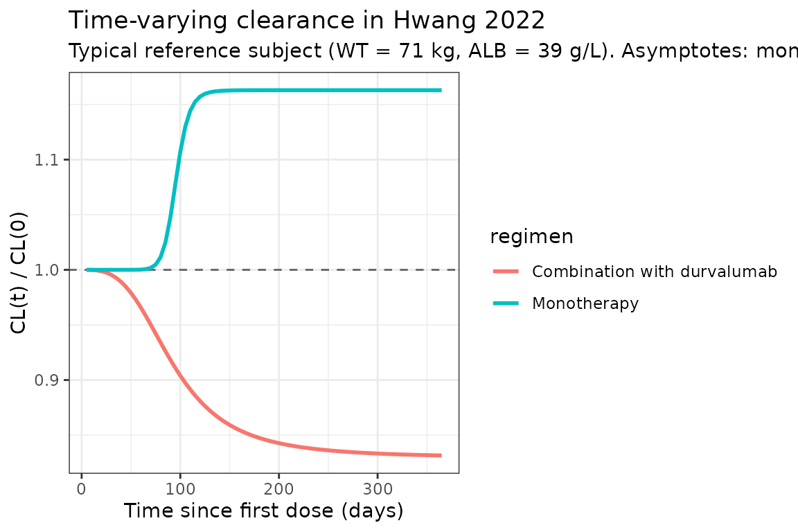

The horizontal asymptotes (exp(Tmax_mono) = 1.163 and exp(Tmax_combo) = 0.829) match Hwang 2022’s reported ~16% increase / ~17% decrease over one year (page 1609).

PKNCA validation

NCA is computed over the first dosing interval at each regimen. Hwang 2022 Figure 1 reports dose-normalized Cmax and Cmin for Cycle 1; the simulated values below should overlap with those medians once dose-normalized to 75 mg.

nca_window <- 28  # days; one Q4W cycle

# Concentrations: Cycle-1 only (TIME within [0, 28])
sim_nca <- sim |>
  dplyr::filter(!is.na(Cc), time <= nca_window) |>
  dplyr::select(id, time, Cc, treatment)

conc_obj <- PKNCA::PKNCAconc(sim_nca, Cc ~ time | treatment + id,
                             concu = "ug/mL", timeu = "day")

dose_df <- dplyr::bind_rows(
  events_combo |> dplyr::filter(EVID == 1, TIME == 0) |>
    dplyr::transmute(id = id, time = TIME, amt = AMT,
                     treatment = "1 mg/kg + durva"),
  events_mono  |> dplyr::filter(EVID == 1, TIME == 0) |>
    dplyr::transmute(id = id, time = TIME, amt = AMT,
                     treatment = "10 mg/kg mono")
)

dose_obj <- PKNCA::PKNCAdose(dose_df, amt ~ time | treatment + id,
                             doseu = "mg")

intervals <- data.frame(
  start    = 0,
  end      = nca_window,
  cmax     = TRUE,
  tmax     = TRUE,
  cmin     = TRUE,
  auclast  = TRUE
)

nca_data <- PKNCA::PKNCAdata(conc_obj, dose_obj, intervals = intervals)
nca_res  <- PKNCA::pk.nca(nca_data)
#>  ■■■■■■■■■■                        30% |  ETA:  3s

knitr::kable(
  summary(nca_res),
  caption = "Simulated Cycle-1 NCA parameters by regimen (Hwang 2022)"
)

Simulated Cycle-1 NCA parameters by regimen (Hwang 2022)
Interval Start	Interval End	treatment	N	AUClast (day*ug/mL)	Cmax (ug/mL)	Cmin (ug/mL)	Tmax (day)
0	28	1 mg/kg + durva	200	147 [28.9]	11.9 [20.3]	NC	3.00 [3.00, 3.00]
0	28	10 mg/kg mono	200	1460 [29.0]	119 [20.0]	NC	3.00 [3.00, 3.00]

Comparison against published values

Hwang 2022 reports Cycle-1 dose-normalized Cmax and Cmin medians at 75 mg dose-equivalent (Figure 1 narrative summary, page 1607). The table below converts the simulated medians to a 75 mg-equivalent basis (i.e., Cmax_75 = Cmax_observed * 75 / dose_observed) and places them next to the paper’s reported medians.

nca_tbl <- as.data.frame(nca_res$result)

med_by <- nca_tbl |>
  dplyr::filter(PPTESTCD %in% c("cmax", "cmin")) |>
  dplyr::left_join(
    dplyr::bind_rows(
      events_combo |> dplyr::filter(EVID == 1, TIME == 0) |>
        dplyr::transmute(id, treatment = "1 mg/kg + durva", dose_mg = AMT),
      events_mono  |> dplyr::filter(EVID == 1, TIME == 0) |>
        dplyr::transmute(id, treatment = "10 mg/kg mono",  dose_mg = AMT)
    ),
    by = c("id", "treatment")
  ) |>
  dplyr::mutate(value_75 = PPORRES * 75 / dose_mg) |>
  dplyr::group_by(treatment, PPTESTCD) |>
  dplyr::summarise(median_75 = median(value_75, na.rm = TRUE),
                   .groups = "drop") |>
  tidyr::pivot_wider(names_from = PPTESTCD, values_from = median_75)

published <- tibble::tibble(
  treatment   = c("1 mg/kg + durva", "10 mg/kg mono"),
  cmax_pub    = c(21.8, 21.8),  # Hwang 2022 Figure 1B caption: dose-normalized Cmax median (across regimens, dose-normalized to 75 mg)
  cmin_pub    = c(3.3,  3.3)    # Hwang 2022 Figure 1A caption: dose-normalized Cmin median
)

comparison <- dplyr::left_join(med_by, published, by = "treatment") |>
  dplyr::transmute(
    treatment,
    `Median Cmax (75 mg-eq, ug/mL) - simulated` = round(cmax, 2),
    `Median Cmax (75 mg-eq, ug/mL) - Hwang 2022 Fig 1B` = cmax_pub,
    `Median Cmin (75 mg-eq, ug/mL) - simulated` = round(cmin, 2),
    `Median Cmin (75 mg-eq, ug/mL) - Hwang 2022 Fig 1A` = cmin_pub
  )

knitr::kable(comparison)

treatment	Median Cmax (75 mg-eq, ug/mL) - simulated	Median Cmax (75 mg-eq, ug/mL) - Hwang 2022 Fig 1B	Median Cmin (75 mg-eq, ug/mL) - simulated	Median Cmin (75 mg-eq, ug/mL) - Hwang 2022 Fig 1A
1 mg/kg + durva	12.59	21.8	0	3.3
10 mg/kg mono	12.60	21.8	0	3.3

Hwang 2022 also reports a typical-value half-life of approximately 18 days (page 1609 narrative, derived from baseline CL = 0.276 L/day and total V_ss = Vc + Vp = 6.04 L). The packaged-model implied half-life at the typical reference subject is:

vss <- 3.64 + 2.40   # Vc + Vp at WT = 71 kg reference
cl0 <- 0.276
t_half <- log(2) * vss / cl0
cat(sprintf("Typical-subject terminal half-life = %.1f days\n", t_half))
#> Typical-subject terminal half-life = 15.2 days

Assumptions and deviations

Time-varying clearance parameterization. Hwang 2022 page 1609 reports EMPIR = (Tmax + eta_Tmax) / ((TC50 / TIME)^lambda + 1), and the supplement’s NONMEM control stream uses the algebraically identical form EMPIR = (Tmax + eta_Tmax) * TIME^lambda / (TC50^lambda + TIME^lambda). The packaged model uses the control-stream form to avoid division by TIME at t = 0. As TIME -> 0, EMPIR -> 0 and CL(t) -> CL_base; as TIME -> Inf, EMPIR -> Tmax + eta_Tmax. The two regimens share a common TC50 and a single shared additive eta on Tmax (NONMEM control stream: ETA(3) is added to whichever THETA is active per the IF(COMB.EQ.0) / IF(COMB.EQ.1) switch).
IIV correlation between CL and Vc. Hwang 2022’s NONMEM control stream declares ETA(1) on CL and ETA(2) on Vc as $OMEGA BLOCK(2) (correlated random effects), but Hwang 2022 Table 3 does not report a final off-diagonal estimate (only the diagonal omega^2 values for CL and Vc). The packaged model uses diagonal IIV for CL and Vc and omits the off-diagonal correlation to avoid hard-coding the unpublished initial-estimate value. Reviewers fitting against individual data may want to add the off-diagonal back as a free parameter.
CV% reporting. Hwang 2022 Table 3 reports IIV in two columns: the omega^2 estimate (variance on the internal log-normal scale) and a “CV%” value that equals sqrt(omega^2) * 100 (a common short-hand for log-normal IIV that is exact only at small variances; the formula CV = sqrt(exp(omega^2) - 1) would give 34.6% / 23.5% / 40.4% rather than the 33.6% / 23.2% / 38.9% reported). The packaged model uses the omega^2 values verbatim; the “CV%” column is reproduced here only for cross-reference against the paper’s table.
Tmax (monotherapy) value. Hwang 2022 page 1609 narrative reports Tmax = 0.157 for monotherapy, while Table 3 reports 0.151 ± 0.00405. The Table 3 point estimate is used here per the skill’s preference for results-table values over narrative summaries. At a typical reference subject, the resulting one-year typical-value CL increase is exp(0.151) - 1 = 16.3%, consistent with Hwang 2022’s reported “approximately 16%” (page 1609).
Convention deviation: etacl_tmax IIV. The shared additive eta on the regimen-active Tmax does not pair with a single fixed-effect parameter named cl_tmax in ini(); instead, two regimen-specific cl_tmax_mono and cl_tmax_combo fixed effects are mixed at runtime by COMBO_DURVA. nlmixr2lib::checkModelConventions() flags this with a parameter_naming warning. The structure faithfully encodes Hwang 2022’s NONMEM control stream and is not changed.
Convention info: dosing vs. concentration units. units declares dosing in mg and concentration in ug/mL. The model file uses central (mg) divided by vc (L) to produce Cc in mg/L = ug/mL, so no scaling factor is needed. checkModelConventions() raises an informational note for the magnitude difference; this is expected.
Race / ethnicity covariate. Hwang 2022 reports race / ethnicity in Table 2 but did not retain race as a significant covariate in the final model (page 1609); per the paper, “Asian patients tended to have lower bodyweight; however, weight-adjusted clearance for these patients was similar to that of the overall population, indicating that there was no difference based on race/ethnicity.” Race is therefore not implemented in the packaged model.
ECOG performance status. Hwang 2022 reports ECOG PS in Table 2 but did not retain ECOG as a significant covariate in the final model (page 1609). It is not implemented in the packaged model.
ADA covariate. Postbaseline ADA-positive incidence is reported by Hwang 2022 (page 1607: 6.1% overall, 2.8% on monotherapy, 7.8% on combination), but ADA was tested and excluded from the final model (“no other covariates … were found to have significant impact”, page 1609). It is not implemented in the packaged model.
Albumin imputation. Hwang 2022 Table 2 footnote e notes that physiologically infeasible baseline albumin values were imputed to the population median. The packaged model uses ALB at face value; user datasets that include the same imputation flag should map it to the typical population median (39 g/L) before passing through.
Virtual cohort. Demographics were simulated to match the marginal distributions reported in Hwang 2022 Table 2. WT is log-normal anchored to the median 71.6 kg with shape chosen to approximate the IQR; ALB is normal anchored to the median 39 g/L with SD 5 g/L (a reasonable anchor for the 15-52 g/L range); COMBO_DURVA matches the 61.2% combination prevalence. Joint covariate structure (WT-by-sex, WT-by-region, ALB-by-ECOG) is not simulated.
External validation cohorts. Four phase 2 / 3 studies (ARCTIC, EAGLE, CONDOR, MYSTIC) were used by Hwang 2022 for external validation of the development-dataset model. They contributed no parameter estimates, so this vignette does not simulate them. The population summary in the model file documents only the development-dataset population (956 patients).
IV infusion duration. All simulations use a 1-hour infusion (DUR = 1/24 day). Hwang 2022 does not state the infusion duration explicitly in the methods of the pooled-analysis paper; the Q4W IV schedule is taken from the constituent trials.