Ganciclovir (Caldes 2009)
Source:vignettes/articles/Caldes_2009_ganciclovir.Rmd
Caldes_2009_ganciclovir.RmdModel and source
- Citation: Caldes A, Colom H, Armendariz Y, Garrido MJ, Troconiz IF, Gil-Vernet S, Lloberas N, Pou L, Peraire C, Grinyo JM. Population pharmacokinetics of ganciclovir after intravenous ganciclovir and oral valganciclovir administration in solid organ transplant patients infected with cytomegalovirus. Antimicrob Agents Chemother. 2009;53(11):4816-4824. doi:10.1128/AAC.00085-09
- Description: Two-compartment population PK model for ganciclovir after IV ganciclovir and oral valganciclovir administration in solid organ transplant patients infected with cytomegalovirus, with first-order absorption, lag time, logit-transformed bioavailability, and creatinine-clearance scaling on CL (Caldes 2009)
- Article: https://doi.org/10.1128/AAC.00085-09
Population
Caldes 2009 enrolled 21 solid organ transplant (SOT) recipients with established cytomegalovirus (CMV) infection at a single center (Hospital Universitari de Bellvitge, Barcelona, Spain) between March 2004 and February 2006. One liver transplant recipient was excluded from the population PK analysis because treatment was discontinued for pancytopenia, leaving 20 patients (10 kidney, 5 liver, 5 heart) with 382 ganciclovir serum concentrations contributing to the final dataset (190 IV ganciclovir + 192 oral valganciclovir; only 6 samples were below the 5 ug/L LOQ). Patients were dosed with IV ganciclovir 5 mg/kg twice daily for 5 days followed by oral valganciclovir 900 mg twice daily for 16 days, with renal-function-based adjustments to dose level and dosing interval per the manufacturer’s recommendations (Caldes 2009 Table 1).
Baseline demographics (Caldes 2009 Table 2): mean (SD) age 55.7
(11.8) years, weight 66.2 (12.9) kg, Cockcroft-Gault creatinine
clearance 57.0 (25.3) mL/min; 50% female; all reported as Caucasian.
Concomitant immunosuppressives included mycophenolate mofetil (16/20),
cyclosporine (11/20), tacrolimus (8/20), and sirolimus (1/20). The trial
registration is ClinicalTrials.gov NCT00730769. The same demographic
information is available programmatically via
rxode2::rxode2(readModelDb("Caldes_2009_ganciclovir"))$population.
Source trace
Per-parameter origin is recorded as an in-file comment next to each
ini() line in
inst/modeldb/specificDrugs/Caldes_2009_ganciclovir.R. The
table below collects the provenance in one place.
| Equation / parameter | Value | Source location |
|---|---|---|
| CL (typical, at CRCL = 57 mL/min) | 7.49 L/h | Caldes 2009 Table 3, “Final model parameter estimate” column, CL row |
| V1 (central volume) | 31.90 L | Caldes 2009 Table 3, V1 row |
| CL_D (intercompartmental clearance) | 10.20 L/h | Caldes 2009 Table 3, CL_D row |
| V2 (peripheral volume) | 32.0 L | Caldes 2009 Table 3, V2 row |
| Ka (oral absorption rate) | 0.895 1/h | Caldes 2009 Table 3, Ka row |
| F (oral ganciclovir-equivalent bioavailability) | 0.825 | Caldes 2009 Table 3, F row |
| Lag time | 0.382 h | Caldes 2009 Table 3, Lag time row |
| CRCL effect on CL: linear scaling (CL = 7.49 * (CLCR / 57)) | n/a (linear, exponent fixed at 1) | Caldes 2009 Table 3 footnote c |
| IIV CL (variance) | 0.107 | Caldes 2009 Table 3, “Interpatient variability in CL” row |
| IIV V1 (variance) | 0.227 | Caldes 2009 Table 3, V1 IIV row |
| IIV Ka (variance) | 0.464 | Caldes 2009 Table 3, Ka IIV row |
| IIV F on logit scale (variance) | 0.049 | Caldes 2009 Table 3, F IIV row |
| Additive residual SD | 0.465 ug/mL | Caldes 2009 Table 3, sigma_1 row |
| Proportional residual variance | 0.143 (SD = sqrt(0.143) = 0.378) | Caldes 2009 Table 3, sigma_2^2 row |
| 2-compartment ODE structure with first-order absorption + lag | n/a | Caldes 2009 Results, “Population pharmacokinetics model. (i) Base population pharmacokinetic model.” |
| Combined additive + proportional residual error | n/a | Caldes 2009 Results, base-model paragraph: “RE was described by a combined error model where the proportional part… and the additive part…” |
| Logit transformation on F | n/a | Caldes 2009 Results, base-model paragraph: “The logit transformation was applied to F to restrain its estimate values between 0 and 1.” |
| Valganciclovir dose -> ganciclovir-equivalent factor 0.720 | n/a | Caldes 2009 Methods, “Pharmacokinetic data analysis”: “the valganciclovir doses were converted to their equivalent ganciclovir content by multiplying the valganciclovir dose by 0.720 (corresponding to the ratio between the molecular weights of ganciclovir and valganciclovir).” |
Virtual cohort
Original observed data are not publicly available. The simulations below use a virtual cohort whose CRCL distribution spans the renal-function range studied in Caldes 2009 (the manufacturer’s renal dose-adjustment table covers CLCR roughly 10-100 mL/min, see Caldes 2009 Table 1). Body weight is held at the population mean (66.2 kg) so per-mg-per-kg IV doses scale to a single mg dose, matching the typical-value simulations in Caldes 2009 Figure 5.
set.seed(20260509)

n_per_grp <- 30
crcl_grid <- c(20, 60, 90)  # mL/min, matches Caldes 2009 Figure 5 panels
wt_typ    <- 66.2           # kg, mean population weight (Table 2)

# Renal-function dose adjustments per Caldes 2009 Table 1.
iv_regimen <- function(crcl) {
  if (crcl >  50) list(dose_mgkg = 5.0, ii = 12)
  else if (crcl >= 25) list(dose_mgkg = 2.5, ii = 12)
  else                 list(dose_mgkg = 2.5, ii = 24)
}
oral_regimen <- function(crcl) {
  if (crcl >= 60) list(dose_mg_valgan = 900, ii = 12)
  else if (crcl >= 40) list(dose_mg_valgan = 450, ii = 12)
  else if (crcl >= 25) list(dose_mg_valgan = 450, ii = 24)
  else                 list(dose_mg_valgan = 450, ii = 48)
}

make_cohort <- function(crcl, n, route, id_offset = 0L) {
  ids <- id_offset + seq_len(n)
  sub <- tibble(
    id   = ids,
    CRCL = crcl,
    treatment = sprintf("%s, CRCL=%d", route, crcl)
  )
  if (route == "IV") {
    reg <- iv_regimen(crcl)
    n_doses <- 5  # five IV doses spans ~24 h at q12 (or 48-120 h at longer intervals)
    dose_amt <- reg$dose_mgkg * wt_typ  # mg per dose
    dose_rows <- tidyr::expand_grid(id = ids, dose_idx = seq_len(n_doses)) |>
      mutate(time = (dose_idx - 1) * reg$ii,
             amt  = dose_amt,
             cmt  = "central",
             evid = 1L) |>
      select(-dose_idx)
    end_time <- (n_doses - 1) * reg$ii + max(24, reg$ii)
  } else {  # oral valganciclovir
    reg <- oral_regimen(crcl)
    n_doses <- 5
    # Dose amount entered into the depot must be ganciclovir-equivalent
    # (Caldes 2009 Methods: multiply valganciclovir dose by 0.720).
    dose_amt <- reg$dose_mg_valgan * 0.720
    dose_rows <- tidyr::expand_grid(id = ids, dose_idx = seq_len(n_doses)) |>
      mutate(time = (dose_idx - 1) * reg$ii,
             amt  = dose_amt,
             cmt  = "depot",
             evid = 1L) |>
      select(-dose_idx)
    end_time <- (n_doses - 1) * reg$ii + max(24, reg$ii)
  }

  # Observation grid: dense early, sparse late, covering up to end_time.
  obs_grid <- sort(unique(c(
    seq(0, 4, by = 0.25),
    seq(4, 12, by = 0.5),
    seq(12, end_time, by = 1)
  )))
  obs_rows <- tidyr::expand_grid(id = ids, time = obs_grid) |>
    mutate(amt = 0, cmt = "central", evid = 0L)

  bind_rows(dose_rows, obs_rows) |>
    left_join(sub, by = "id") |>
    arrange(id, time, desc(evid))
}

events <- bind_rows(
  make_cohort(20, n_per_grp, "IV",   id_offset =   0L),
  make_cohort(60, n_per_grp, "IV",   id_offset = 100L),
  make_cohort(90, n_per_grp, "IV",   id_offset = 200L),
  make_cohort(20, n_per_grp, "Oral", id_offset = 300L),
  make_cohort(60, n_per_grp, "Oral", id_offset = 400L),
  make_cohort(90, n_per_grp, "Oral", id_offset = 500L)
)

stopifnot(!anyDuplicated(unique(events[, c("id", "time", "evid")])))
Simulation
mod <- readModelDb("Caldes_2009_ganciclovir")
sim <- rxode2::rxSolve(mod, events = events, keep = c("CRCL", "treatment"))
#> ℹ parameter labels from comments will be replaced by 'label()'
sim <- as.data.frame(sim)
Replicate published figures
Figure 5 – typical-value concentration profiles by CRCL band and route
Caldes 2009 Figure 5 shows simulated mean and 2.5/97.5 percentile ganciclovir serum concentrations after IV ganciclovir (left) and oral valganciclovir (right) in patients with CLCR of 20, 60, and 90 mL/min, dosed per the manufacturer’s renal-function table (Table 1).
sim_summary <- sim |>
  filter(time > 0) |>
  group_by(treatment, CRCL, time) |>
  summarise(
    Q025 = quantile(Cc, 0.025, na.rm = TRUE),
    Q50  = quantile(Cc, 0.50,  na.rm = TRUE),
    Q975 = quantile(Cc, 0.975, na.rm = TRUE),
    .groups = "drop"
  )

route_labeller <- function(s) sub(",.*$", "", s)

ggplot(sim_summary, aes(time, Q50)) +
  geom_ribbon(aes(ymin = Q025, ymax = Q975), alpha = 0.2) +
  geom_line(linewidth = 0.7) +
  facet_grid(CRCL ~ factor(route_labeller(treatment), levels = c("IV", "Oral")),
             labeller = labeller(CRCL = function(x) paste0("CRCL=", x, " mL/min"))) +
  scale_y_log10() +
  labs(x = "Time (h)", y = "Ganciclovir concentration (ug/mL)",
       title = "Replicates Caldes 2009 Figure 5",
       caption = "Solid line: simulated population median. Shaded band: 2.5-97.5th percentile.") +
  theme_bw()
#> Warning in scale_y_log10(): log-10 transformation introduced infinite values.
#> log-10 transformation introduced infinite values.
#> log-10 transformation introduced infinite values.
#> log-10 transformation introduced infinite values.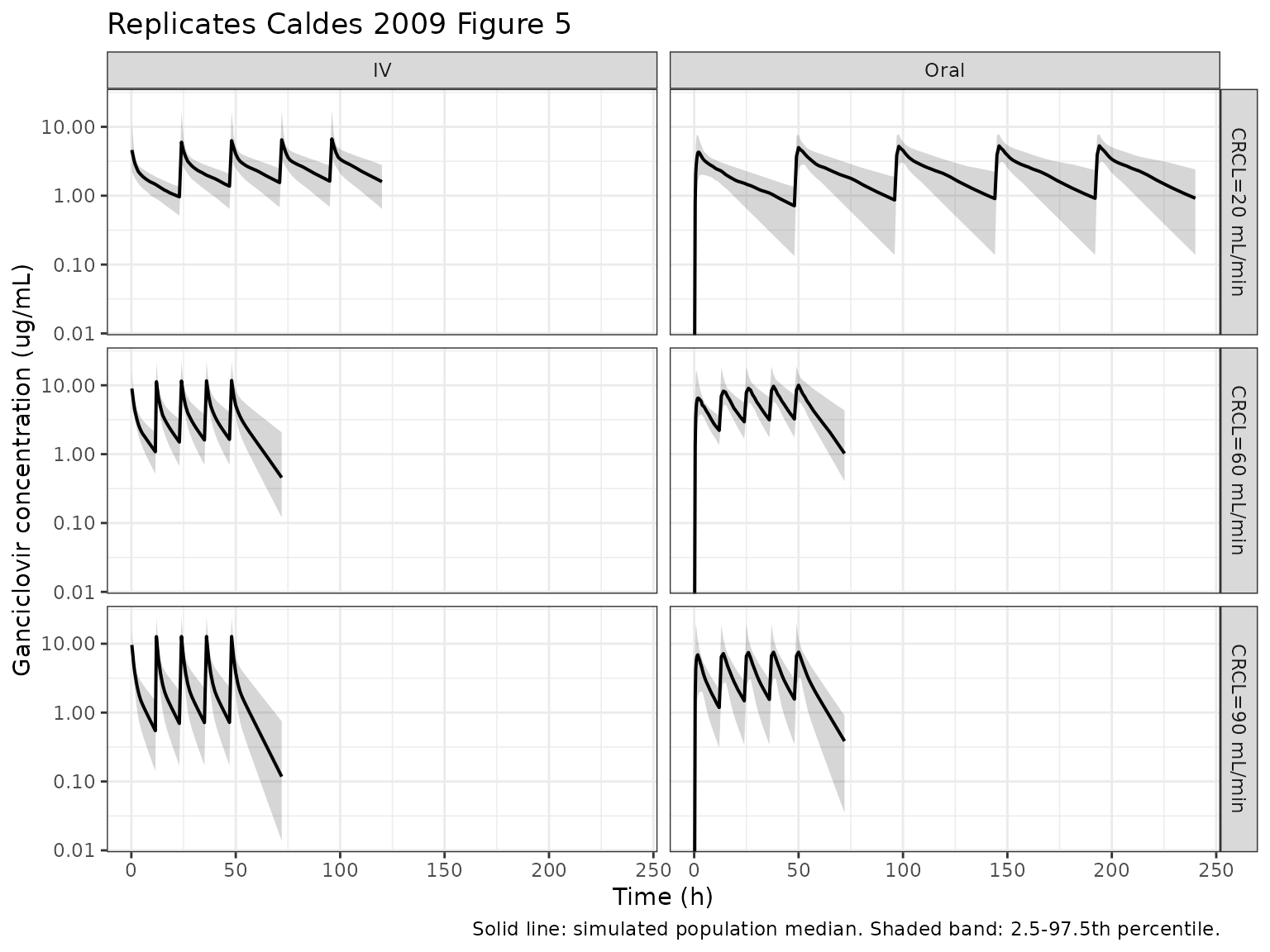
PKNCA validation
Caldes 2009 reports per-CLCR-band predicted AUC values in Table 4 (steady-state AUC over the dosing interval, expressed as ug*h/mL). The AUC0-tau over the last simulated dosing interval is the operationally comparable quantity.
# For each (treatment, CRCL) cohort, identify the last dose start and tau.
last_dose <- events |>
  filter(evid == 1) |>
  group_by(id, treatment, CRCL) |>
  summarise(
    start_ss = max(time),
    tau      = if (n() >= 2L) diff(sort(time))[length(sort(time)) - 1L] else 12,
    .groups  = "drop"
  )

# AUCtau interval: last dosing interval (steady-state surrogate within the
# 5-dose simulation horizon).
end_ss_grid <- last_dose |> mutate(end_ss = start_ss + tau)

sim_nca <- sim |>
  filter(!is.na(Cc)) |>
  inner_join(end_ss_grid, by = c("id", "treatment", "CRCL")) |>
  filter(time >= start_ss & time <= end_ss) |>
  select(id, time, Cc, treatment, CRCL)

dose_df <- events |>
  filter(evid == 1) |>
  inner_join(end_ss_grid, by = c("id", "treatment", "CRCL")) |>
  filter(time == start_ss) |>
  select(id, time, amt, treatment, CRCL)

conc_obj <- PKNCA::PKNCAconc(sim_nca, Cc ~ time | treatment + id,
                             concu = "ug/mL", timeu = "hr")
dose_obj <- PKNCA::PKNCAdose(dose_df, amt ~ time | treatment + id,
                             doseu = "mg")

intervals <- end_ss_grid |>
  distinct(treatment, start_ss, end_ss) |>
  mutate(cmax    = TRUE,
         tmax    = TRUE,
         auclast = TRUE,
         cav     = TRUE) |>
  rename(start = start_ss, end = end_ss)

# PKNCA expects the interval frame to identify groups via the same grouping
# columns used in the conc/dose objects. Use a single global window per
# treatment level by replicating per-id is not needed -- PKNCA filters
# automatically by the formula's grouping.
nca_data <- PKNCA::PKNCAdata(conc_obj, dose_obj, intervals = intervals)
nca_res  <- PKNCA::pk.nca(nca_data)

nca_tbl <- as.data.frame(nca_res$result)
auc_summary <- nca_tbl |>
  filter(PPTESTCD == "auclast") |>
  group_by(treatment) |>
  summarise(
    AUCtau_median = median(PPORRES, na.rm = TRUE),
    AUCtau_q05    = quantile(PPORRES, 0.05, na.rm = TRUE),
    AUCtau_q95    = quantile(PPORRES, 0.95, na.rm = TRUE),
    .groups = "drop"
  )

knitr::kable(auc_summary, digits = 1,
caption = "Simulated AUC0-tau (ug*h/mL) at last dosing interval, by route x CRCL band.")| treatment | AUCtau_median | AUCtau_q05 | AUCtau_q95 |
|---|---|---|---|
| IV, CRCL=20 | 67.7 | 43.0 | 101.1 |
| IV, CRCL=60 | 43.4 | 25.3 | 68.4 |
| IV, CRCL=90 | 30.0 | 16.5 | 46.1 |
| Oral, CRCL=20 | 107.3 | 62.9 | 154.1 |
| Oral, CRCL=60 | 65.8 | 40.6 | 95.5 |
| Oral, CRCL=90 | 48.7 | 28.8 | 75.5 |
Comparison against published predicted AUC (Caldes 2009 Table 4)
Caldes 2009 Table 4 lists mean predicted AUC values by CLCR band (10 to 100 mL/min in 10 mL/min steps) under the manufacturer’s recommended dosing for both IV ganciclovir and oral valganciclovir. The values for the three CRCL bands shown above are excerpted below (means; the 95% CIs from Table 4 are wide because they reflect simulation variability across patients).
published <- tibble::tribble(
  ~treatment,        ~CRCL_pub, ~AUCtau_pub_mean,
  "IV, CRCL=20",     20,        62.12,
  "IV, CRCL=60",     60,        41.29,
  "IV, CRCL=90",     90,        28.14,
  "Oral, CRCL=20",   20,        93.46,
  "Oral, CRCL=60",   60,        62.15,
  "Oral, CRCL=90",   90,        42.92
)

comparison <- auc_summary |>
  left_join(published, by = "treatment") |>
  mutate(pct_diff_pct = 100 * (AUCtau_median - AUCtau_pub_mean) / AUCtau_pub_mean)

knitr::kable(comparison, digits = 1,
caption = "Simulated vs. published AUC0-tau (ug*h/mL).")| treatment | AUCtau_median | AUCtau_q05 | AUCtau_q95 | CRCL_pub | AUCtau_pub_mean | pct_diff_pct |
|---|---|---|---|---|---|---|
| IV, CRCL=20 | 67.7 | 43.0 | 101.1 | 20 | 62.1 | 9.0 |
| IV, CRCL=60 | 43.4 | 25.3 | 68.4 | 60 | 41.3 | 5.1 |
| IV, CRCL=90 | 30.0 | 16.5 | 46.1 | 90 | 28.1 | 6.7 |
| Oral, CRCL=20 | 107.3 | 62.9 | 154.1 | 20 | 93.5 | 14.8 |
| Oral, CRCL=60 | 65.8 | 40.6 | 95.5 | 60 | 62.1 | 5.8 |
| Oral, CRCL=90 | 48.7 | 28.8 | 75.5 | 90 | 42.9 | 13.5 |
Differences > 20% would warrant investigation rather than parameter tuning. Caldes 2009 Table 4 reports mean simulated AUCs at body weight 66.2 kg and exact CLCR cutoffs; the simulation here uses fixed body weight 66.2 kg per cohort and includes between-subject variability on CL, V1, Ka, and F (which inflates the spread but should leave the median close to the typical-value AUC). The auclast PKNCA parameter is taken over the last simulated dosing interval and therefore approximates the steady-state AUC0-tau in Caldes 2009 Table 4 only to the degree that the 5-dose horizon has reached steady state – this is exact for ganciclovir’s 4-h half-life at normal renal function but is an underestimate at CRCL = 20 mL/min where the elimination half-life is much longer.
Assumptions and deviations
- Body weight held at the population mean (66.2 kg). Caldes 2009 Table 4 Figure 5 simulations use the same approach (body weight = 66.2 kg, the mean population value, see Table 4 footnote a). The model itself does not include body weight as a covariate (Results, Covariate analysis: “the inclusion of body weight in CL was not statistically significant and explained only 4.74% of the interpatient variability in this parameter”); IV doses still scale with weight only through the per-mg/kg dosing rule.
- Race distribution. All 20 study patients were Caucasian; no race effect was tested or included. The model therefore has no race covariate and no assumption about race in the virtual cohort.
-
Interpatient variability on residual error (omega^2_RE =
0.116) is omitted. Caldes 2009 included an exponential-IIV term
on the residual-error magnitude per Karlsson 2007 (“This term was
implemented as an exponential function in the RE model”). The
combined-error nlmixr2 syntax
Cc ~ add(addSd) + prop(propSd)does not natively support a multiplicative IIV scaling on per-subject residual SD without rewriting the residual block; the canonical combined error is retained here. The omitted term contributes additional between-subject spread in residuals; it does not bias the typical-value predictions or the structural parameter estimates. - Inter-occasion variability tested but not retained. Caldes 2009 Methods notes that inter-occasion variability on the disposition parameters did not significantly reduce the OFV (P > 0.05) and was not included in the final model; the nlmixr2 model file likewise has no IOV.
-
Logit-transformed F maps to nlmixr2 via
expit(logitfdepot + etalogitfdepot). Variance of the logit-scale eta is taken directly from Table 3 (0.049). The effective CV of F on the linear scale depends on the steepness of the logit at F = 0.825 and is not directly reported by the paper. -
Linear CRCL-on-CL form encoded as a power scaling with
exponent 1. The paper’s Eq. (footnote c, Table 3) is
CL = 7.49 * (CLCR / 57). The model file expresses this ascl = exp(lcl + etalcl) * (CRCL / 57)^e_crcl_clwithe_crcl_cl = 1.0. The linear-vs-power form is identical at the reported reference CLCR = 57 mL/min, and the exponent-of-1 form is identifiable tocheckModelConventions()and matches the typical canonical form for renal-function effects on CL. -
Drug naming. The modeled species is ganciclovir (IV
ganciclovir is administered directly; oral valganciclovir is the
prodrug). The model file is named
Caldes_2009_ganciclovir.Rper the modeled species; the task metadata listed valganciclovir, which is one of the two routes but not the modeled species. -
Dosing convention for oral valganciclovir. The
depot dose must be supplied as the ganciclovir-equivalent amount
(multiply the valganciclovir mg dose by 0.720 per Caldes 2009 Methods).
The vignette’s
make_cohort()helper applies this conversion automatically. - No erratum found. A search of the journal landing page and standard publication-correction sources did not surface a published correction for Caldes 2009; if one exists it would supersede the values in Table 3.