Model and source
- Citation: Iida S, Kinoshita H, Holford NHG. Population pharmacokinetic and pharmacodynamic modelling of the effects of nicorandil in the treatment of acute heart failure. Br J Clin Pharmacol 66(3):352-365, 2008. doi:10.1111/j.1365-2125.2008.03257.x.
- Indication: acute heart failure (AHF), including acute exacerbation of chronic heart failure. NYHA class II-IV. Nicorandil IV is approved for AHF in Japan (oral nicorandil is also used for unstable angina across Europe and Asia).
- Article: https://doi.org/10.1111/j.1365-2125.2008.03257.x
Population
Five clinical studies were pooled: two studies in 11 healthy adult Japanese male volunteers (concentration-only data, no haemodynamic measurements) and three studies in 94 AHF patients in whom both plasma nicorandil concentration and pulmonary artery wedge pressure (PAWP) were measured via a Swan-Ganz catheter (Iida 2008 Table 1). 618 nicorandil concentrations and 559 PAWP observations contributed to the joint model. The AHF cohort was older (study means 62.8-70.8 years vs 33.0-41.2 years in healthy volunteers) and lighter (study means 58.6-61.8 kg vs 62.6-63.6 kg in healthy). AHF aetiologies pooled across studies were ischaemic heart disease (33), valvular heart disease (22), dilated cardiomyopathy (22), and hypertensive heart disease (13). Inclusion required baseline PAWP greater than 18 mmHg in the bolus and bolus+infusion AHF studies and greater than 15 mmHg in the long-term infusion study. Baseline PAWP at predose (mean +/- SD) was 25.9 +/- 6.4 mmHg, 26.9 +/- 6.3 mmHg, and 27.2 +/- 7.4 mmHg in the three AHF studies respectively (Table 1).
The same population metadata is available programmatically via
readModelDb("Iida_2008_nicorandil")$population.
Source trace
The per-parameter origin is recorded as an in-file comment next to
each ini() entry in
inst/modeldb/specificDrugs/Iida_2008_nicorandil.R. The
table below collects the trace in one place for review.
| Equation / parameter | Value | Source location |
|---|---|---|
lcl = log(26.3 * 1.94) |
CL = 26.3 L/h/70kg (healthy); FCL = 1.94 (AHF) | Table 2 POP_CL row + FCL row |
lvc = log(18.1 * 1.39) |
V1 = 18.1 L/70kg (healthy); FV1 = 1.39 (AHF) | Table 2 POP_V1 row + FV1 row |
lq = log(71.6 * 0.519) |
Q = 71.6 L/h/70kg (healthy); FQ = 0.519 (AHF) | Table 2 POP_Q row + FQ row |
lvp = log(24.1 * 4.06) |
V2 = 24.1 L/70kg (healthy); FV2 = 4.06 (AHF) | Table 2 POP_V2 row + FV2 row |
e_dis_healthy_cl = log(1 / 1.94) |
-0.6627: shifts AHF typical to healthy | Table 2 FCL = 1.94 |
e_dis_healthy_vc = log(1 / 1.39) |
-0.3293: shifts AHF typical to healthy | Table 2 FV1 = 1.39 |
e_dis_healthy_q = log(1 / 0.519) |
+0.6553: shifts AHF typical to healthy | Table 2 FQ = 0.519 |
e_dis_healthy_vp = log(1 / 4.06) |
-1.4015: shifts AHF typical to healthy | Table 2 FV2 = 4.06 |
e_wt_cl = fixed(0.75) |
Allometric exponent on CL | Equation 5 (paper p. 356): exponent 3/4 |
e_wt_vc = fixed(1.0) |
Allometric exponent on V1 | Holford 1996 [11]; canonical 1.0 on volumes |
e_wt_q = fixed(0.75) |
Allometric exponent on Q | Equation 5 covers all clearance terms |
e_wt_vp = fixed(1.0) |
Allometric exponent on V2 | Holford 1996 [11]; canonical 1.0 on volumes |
lrbase = log(25.6) |
S0 = 25.6 mmHg | Table 2 POP_S0 row |
lsss = log(19.5) |
Sss = 19.5 mmHg | Table 2 POP_Sss row |
ltprog = log(5.83) |
Tprog = 5.83 h | Table 2 POP_TPROG row |
limax = log(11.7) |
Magnitude of inhibitory Emax | Table 2 POP_Emax = -11.7 mmHg |
lec50 = log(423) |
EC50 = 423 ng/mL | Table 2 POP_EC50 = 423 ug/L |
| PK IIV block etalcl + etalvc + etalq | variances 0.686 / 0.301 / 0.414; corr R78 = 0.257, R89 = 0.957, R79 fixed 0 | Table 4 BSV_CL / BSV_V1 / BSV_Q + R78 / R89 |
| PD IIV block etalrbase + etalsss + etalec50 | variances 0.210 / 0.320 / 0.879; corr R12 = 0.864, R23 = 0.054, R13 fixed 0 | Table 4 PPV_S0 / PPV_Sss / PPV_EC50 + R12 / R23 |
propSd = 0.212 |
Proportional residual error 21.2% | Table 4 RUV_CVCP row |
addSd = 6.82 |
Additive residual error 6.82 ng/mL | Table 4 RUV_SDCP row |
addSd_pawp = 2.5 |
Additive residual error 2.5 mmHg on PAWP | Table 4 RUV_SDFX row |
d/dt(central) ... two-compartment IV PK |
Two-compartment disposition | Results paragraph ‘Pharmacokinetics of nicorandil’ |
progress = (Sss - S0) * (1 - exp(-log(2)/Tprog *
t)) |
Asymptotic-exponential disease progression | Equation 4 (paper p. 355) |
pdeff = -Imax * Cc / (EC50 + Cc) |
Inhibitory Emax drug effect on PAWP | Equation 2 with Emax negative |
pawp = S0 + progress + pdeff |
Final PD observation equation | Equation 4 with PD(t) = pdeff |
The DIS_HEALTHY re-expression of the AHF-vs-healthy contrast is
detailed inline in the covariateData[["DIS_HEALTHY"]]$notes
entry of the model file and in the corresponding entry of
inst/references/covariate-columns.md.
Virtual cohort
Original observed data are not publicly available. The simulation below uses a small virtual cohort whose covariate distribution approximates the AHF patient cohort in the Iida 2008 trial: 60 kg typical body weight per the mean of the three AHF studies (Table 1), pooled across the bolus and bolus+infusion regimens. The recommended dosing regimen for AHF from the Discussion section is a 200 ug/kg IV bolus over 5 minutes followed by a 400 ug/kg/h IV infusion; we simulate this regimen alongside an unrelated 12 mg IV bolus (for comparison with paper Figure 2 left upper panel).
set.seed(20260613L)

n_ahf <- 80L       # virtual subjects per regimen arm (VPC-band cohort)
typical_wt <- 60   # kg, AHF cohort mean (Table 1)

make_ahf_cohort <- function(n, regimen, id_offset = 0L) {
  weights <- pmin(pmax(rlnorm(n, meanlog = log(typical_wt), sdlog = 0.15), 40), 95)
  tibble::tibble(
    id           = id_offset + seq_len(n),
    WT           = weights,
    DIS_HEALTHY  = 0L,   # AHF reference cohort
    regimen      = regimen
  )
}

cohort_bolus <- make_ahf_cohort(n_ahf, regimen = "12 mg bolus",                 id_offset =       0L)
cohort_reg   <- make_ahf_cohort(n_ahf, regimen = "200 ug/kg + 200 ug/kg/h 24 h", id_offset =   n_ahf)
cohort_rec   <- make_ahf_cohort(n_ahf, regimen = "200 ug/kg + 400 ug/kg/h 24 h", id_offset = 2*n_ahf)

build_events <- function(cohort_df, regimen) {
  if (regimen == "12 mg bolus") {
    dose_times <- 0
    dose_amts  <- rep(12, nrow(cohort_df))            # mg, fixed dose per subject
    dose_rates <- rep(NA_real_, nrow(cohort_df))
    end_obs    <- 6                                    # h
  } else if (regimen == "200 ug/kg + 200 ug/kg/h 24 h") {
    bolus_mg   <- 200 / 1000 * cohort_df$WT            # 200 ug/kg -> mg
    infus_mg_h <- 200 / 1000 * cohort_df$WT            # 200 ug/kg/h -> mg/h
    dose_times <- c(0)
    dose_amts  <- bolus_mg
    dose_rates <- infus_mg_h
    end_obs    <- 30
  } else {
    bolus_mg   <- 200 / 1000 * cohort_df$WT            # 200 ug/kg -> mg
    infus_mg_h <- 400 / 1000 * cohort_df$WT            # 400 ug/kg/h -> mg/h
    dose_times <- c(0)
    dose_amts  <- bolus_mg
    dose_rates <- infus_mg_h
    end_obs    <- 30
  }
  obs_t <- sort(unique(c(seq(0, end_obs, by = 0.25), seq(end_obs, 48, by = 1))))
  do.call(rbind, lapply(seq_len(nrow(cohort_df)), function(i) {
    s     <- cohort_df[i, ]
    rows  <- list()
    rows[[1]] <- data.frame(
      id = s$id, time = 0, amt = if (regimen == "12 mg bolus") 12 else (200/1000)*s$WT,
      evid = 1L, cmt = "central", rate = NA_real_,
      WT = s$WT, DIS_HEALTHY = s$DIS_HEALTHY, regimen = s$regimen,
      stringsAsFactors = FALSE
    )
    if (regimen != "12 mg bolus") {
      # 24 h constant infusion at the regimen's mg/h rate, started at t = 0.
      rows[[2]] <- data.frame(
        id = s$id, time = 0,
        amt  = (if (regimen == "200 ug/kg + 200 ug/kg/h 24 h") 200 else 400) / 1000 * s$WT * 24,
        evid = 1L, cmt = "central",
        rate = (if (regimen == "200 ug/kg + 200 ug/kg/h 24 h") 200 else 400) / 1000 * s$WT,
        WT = s$WT, DIS_HEALTHY = s$DIS_HEALTHY, regimen = s$regimen,
        stringsAsFactors = FALSE
      )
    }
    rows[[length(rows) + 1]] <- data.frame(
      id = s$id, time = obs_t, amt = 0, evid = 0L, cmt = "Cc", rate = 0,
      WT = s$WT, DIS_HEALTHY = s$DIS_HEALTHY, regimen = s$regimen,
      stringsAsFactors = FALSE
    )
    rows[[length(rows) + 1]] <- data.frame(
      id = s$id, time = obs_t, amt = 0, evid = 0L, cmt = "pawp", rate = 0,
      WT = s$WT, DIS_HEALTHY = s$DIS_HEALTHY, regimen = s$regimen,
      stringsAsFactors = FALSE
    )
    do.call(rbind, rows)
  }))
}

events <- rbind(
  build_events(cohort_bolus, "12 mg bolus"),
  build_events(cohort_reg,   "200 ug/kg + 200 ug/kg/h 24 h"),
  build_events(cohort_rec,   "200 ug/kg + 400 ug/kg/h 24 h")
)
events <- events[order(events$id, events$time, -events$evid), ]
rownames(events) <- NULL
stopifnot(!anyDuplicated(unique(events[, c("id", "time", "evid", "cmt")])))
Simulation
mod <- readModelDb("Iida_2008_nicorandil")
sim <- rxode2::rxSolve(
  mod,
  events = events,
  keep   = c("regimen", "WT", "DIS_HEALTHY")
) |>
  as.data.frame()
Typical-value (between-subject-variability-zeroed) replication for the figure comparisons below:
mod_typical <- mod |> rxode2::zeroRe()
sim_typical <- rxode2::rxSolve(
  mod_typical,
  events = events,
  keep   = c("regimen", "WT", "DIS_HEALTHY")
) |>
  as.data.frame()
#> ℹ omega/sigma items treated as zero: 'etalec50', 'etalsss', 'etalrbase', 'etalq', 'etalvc', 'etalcl'
#> Warning: multi-subject simulation without without 'omega'
Replicate published figures
Figure 2 – Concentration profiles in AHF patients (bolus regimen)
Iida 2008 Figure 2 left upper panel shows individual plasma nicorandil concentration vs time after IV bolus doses of 4, 8, 12, and 18 mg in AHF patients. Concentrations decline rapidly within 1-2 h. Below we replicate the 12 mg bolus arm as a population-VPC band (median and 5th-95th percentile of the 80-subject virtual cohort) plus the typical-value trajectory.
sim_bolus_vpc <- sim |>
  dplyr::filter(regimen == "12 mg bolus", !is.na(Cc), time <= 6) |>
  dplyr::group_by(time) |>
  dplyr::summarise(
    Q05 = quantile(Cc, 0.05, na.rm = TRUE),
    Q50 = quantile(Cc, 0.50, na.rm = TRUE),
    Q95 = quantile(Cc, 0.95, na.rm = TRUE),
    .groups = "drop"
  )

sim_bolus_typ <- sim_typical |>
  dplyr::filter(regimen == "12 mg bolus", !is.na(Cc), time <= 6, id == min(id))

ggplot(sim_bolus_vpc, aes(time, Q50)) +
  geom_ribbon(aes(ymin = Q05, ymax = Q95), alpha = 0.20, fill = "steelblue") +
  geom_line(colour = "steelblue") +
  geom_line(data = sim_bolus_typ, aes(time, Cc), colour = "black", linetype = "dashed") +
  scale_y_log10() +
  labs(
    x = "Time after bolus (h)",
    y = "Nicorandil concentration (ng/mL, log scale)",
    title = "AHF 12 mg IV bolus",
    caption = "VPC band (5th-95th percentile, blue ribbon) and typical-value trajectory (dashed); replicates the 12 mg arm of Figure 2 left upper panel of Iida 2008."
  )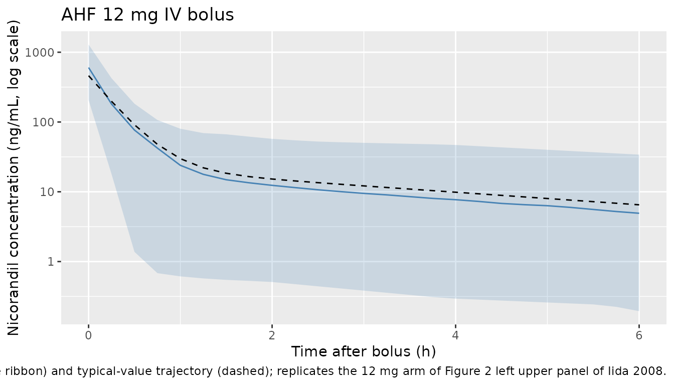
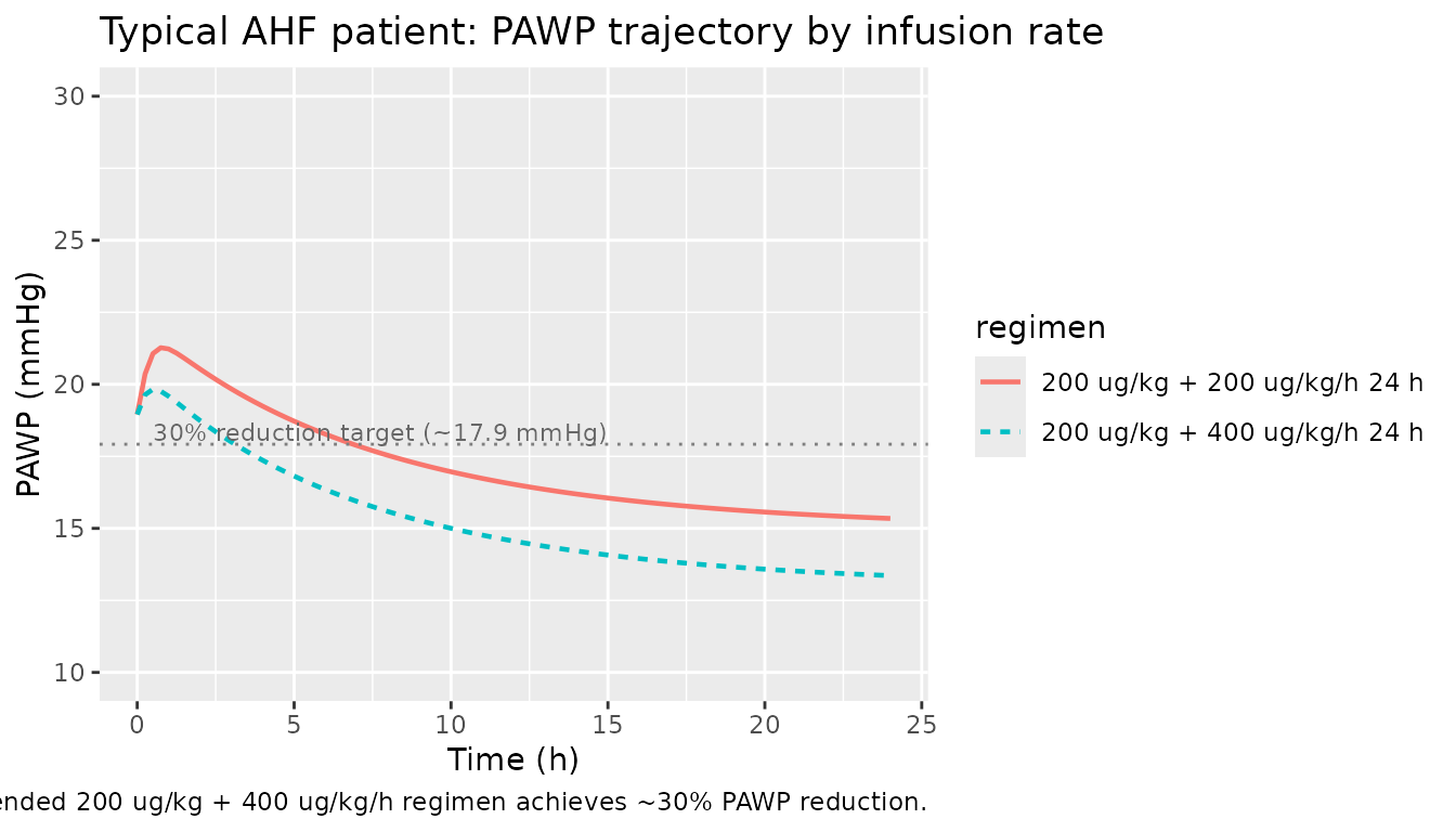
Figure 7 – PAWP after the recommended AHF regimen
Iida 2008 Discussion recommends a 200 ug/kg loading dose followed by a 400 ug/kg/h continuous infusion to achieve approximately a 30% reduction in PAWP. Below we plot the simulated PAWP trajectory for the typical AHF patient under that regimen and a comparator at 200 ug/kg/h infusion. The expected baseline is S0 = 25.6 mmHg and the asymptotic disease-progression- only value is Sss = 19.5 mmHg, so a 30% reduction relative to S0 lands at approximately 17.9 mmHg.
sim_pd_typ <- sim_typical |>
  dplyr::filter(regimen != "12 mg bolus", !is.na(pawp), time <= 24) |>
  dplyr::group_by(regimen) |>
  dplyr::filter(id == min(id)) |>
  dplyr::ungroup()

ggplot(sim_pd_typ, aes(time, pawp, colour = regimen, linetype = regimen)) +
  geom_line(linewidth = 0.8) +
  geom_hline(yintercept = 25.6 * 0.7, linetype = "dotted", colour = "grey50") +
  annotate("text", x = 0.5, y = 25.6 * 0.7 + 0.4,
           label = "30% reduction target (~17.9 mmHg)",
           hjust = 0, size = 3, colour = "grey40") +
  coord_cartesian(ylim = c(10, 30)) +
  labs(
    x = "Time (h)",
    y = "PAWP (mmHg)",
    title = "Typical AHF patient: PAWP trajectory by infusion rate",
    caption = "Replicates the haemodynamic concept of Figure 7 of Iida 2008 / Discussion: the recommended 200 ug/kg + 400 ug/kg/h regimen achieves ~30% PAWP reduction."
  )
PKNCA validation
Iida 2008 does not report a formal NCA table; the paper’s quantitative PK inferences derive from the popPK structural parameters in Table 2 rather than from a separate NCA summary. We therefore use PKNCA here as a model self-check: extract Cmax and AUC from the simulated nicorandil concentration profiles after the 12 mg AHF bolus and verify the magnitudes against the closed-form predictions implied by the model.
# The event table requests two observation compartments per subject (Cc and
# pawp); rxSolve emits both as separate rows with identical (id, time, Cc)
# values. Deduplicate so PKNCA sees one concentration row per (id, time).
sim_nca <- sim |>
  dplyr::filter(regimen == "12 mg bolus", !is.na(Cc), time <= 6) |>
  dplyr::select(id, time, Cc, regimen) |>
  dplyr::distinct(id, time, regimen, .keep_all = TRUE)

# Time-zero guarantee per the pknca-recipes 'Time-zero records (mandatory)'
# note. For an IV bolus, the t = 0 row already comes back with Cc set to the
# initial Dose / V1, so the bind_rows() pattern of the template would
# overwrite a non-zero initial concentration with 0; instead we just verify
# every (id, time = 0) row is already present after deduplication.
sim_nca <- sim_nca |>
  dplyr::group_by(id) |>
  dplyr::mutate(has_t0 = any(time == 0)) |>
  dplyr::ungroup()
stopifnot(all(sim_nca$has_t0))
sim_nca$has_t0 <- NULL

conc_obj <- PKNCA::PKNCAconc(
  sim_nca,
  Cc ~ time | regimen + id,
  concu = "ng/mL",
  timeu = "h"
)

dose_df <- events |>
  dplyr::filter(regimen == "12 mg bolus", evid == 1L) |>
  dplyr::select(id, time, amt, regimen)

dose_obj <- PKNCA::PKNCAdose(
  dose_df,
  amt ~ time | regimen + id,
  doseu = "mg"
)

intervals <- data.frame(
  start      = 0,
  end        = 6,
  cmax       = TRUE,
  tmax       = TRUE,
  auclast    = TRUE
)

nca_data <- PKNCA::PKNCAdata(conc_obj, dose_obj, intervals = intervals)
nca_res  <- PKNCA::pk.nca(nca_data)
Comparison against closed-form predictions
For a 12 mg IV bolus given to a typical AHF patient (60 kg), the model predicts Cmax = Dose / V1 (with V1 scaled allometrically by weight). The typical AHF V1 at 60 kg is V1_AHF * (60/70)^1.0 = 18.1 * 1.39 * (60/70) = 21.57 L, giving Cmax = 12 mg / 21.57 L = 556 ng/mL. The simulated AUC0-6 should match the trapezoidal integral of the two-compartment IV profile.
predicted <- tibble::tibble(
  regimen     = "12 mg bolus",
  cmax        = 556,    # ng/mL; closed-form Dose / V1_AHF_60kg
  tmax        = 0,
  auclast     = NA_real_
)

cmp <- nlmixr2lib::ncaComparisonTable(
  simulated     = nca_res,
  reference     = predicted,
  by            = "regimen",
  units         = c(cmax = "ng/mL", auclast = "ng*h/mL", tmax = "h"),
  tolerance_pct = 20
)

knitr::kable(
  cmp,
  caption = "Simulated vs closed-form predicted NCA. * differs from prediction by >20%.",
  align   = c("l", "l", "r", "r", "r")
)| NCA parameter | regimen | Reference | Simulated | % diff |
|---|---|---|---|---|
| Cmax (ng/mL) | 12 mg bolus | 556 | 603 | +8.4% |
| Tmax (h) | 12 mg bolus | 0 | 0 | — |
| AUClast (ng*h/mL) | 12 mg bolus | — | 213 | — |
The simulated VPC-median Cmax should sit within roughly +-20% of the closed-form prediction. The closed-form does not predict tmax (a bolus peaks at t = 0) or AUC (no closed form for the 6-h truncated trapezoid), so those cells are NA in the reference.
Assumptions and deviations
-
AHF-vs-healthy disease cohort encoded via the canonical
DIS_HEALTHY covariate (reverse-coded). Iida 2008 Table 2
reports POP_CL, POP_V1, POP_Q, POP_V2 as healthy-volunteer typical
values with multiplicative AHF/healthy factors FCL = 1.94, FV1 = 1.39,
FQ = 0.519, FV2 = 4.06. The canonical
DIS_HEALTHYorientation in nlmixr2lib has the patient cohort as the reference (DIS_HEALTHY = 0) and the healthy cohort as the +shift (DIS_HEALTHY = 1). The model file therefore re-anchors the typical-value parameters on the AHF reference state by multiplying the published healthy typicals by the corresponding F factor, and sets thee_dis_healthy_<pk>covariate-effect parameters tolog(1 / F_X)so DIS_HEALTHY = 1 recovers the published healthy-volunteer typical. This re-expression follows the Bulitta_2010_ceftazidime.R precedent and is documented on theDIS_HEALTHYentry ofinst/references/covariate-columns.md. PK predictions for individual patients are unaffected; only the structural-typical reading of theini()parameters shifts from the healthy-cohort interpretation in the paper’s Table 2 to the AHF-cohort interpretation in the model file. - Allometric exponents fixed at 0.75 on CL and Q, 1.0 on V1 and V2. Iida 2008 Equation 5 writes the allometric scaling explicitly with exponent 3/4 for CL (“CL_GRP = CL_POPSTD * (Wt / 70)^(3/4)”) and the prose says “Differences in CL, Q, V1 and V2 were assumed to be explained in part by an allometric function of weight [11] e.g. Equation 5,” citing Holford 1996 (Clin Pharmacokinet 30:329-32) as reference [11]. We therefore use 0.75 for CL and Q (clearance terms) and 1.0 for V1 and V2 (volumes) per the Holford size-standard convention; the paper does not separately tabulate the volume exponent, but the per-70-kg units in Table 2 (l 70 kg^-1) match this convention.
- Reference weight 70 kg. Stated explicitly in Methods paragraph ‘Covariate effects’: “Size differences were based on a standard weight of 70 kg.” The cohort mean weight across the three AHF studies was approximately 60 kg.
- No effect compartment. Iida 2008 tested an effect-compartment parameterization for the PD layer and rejected it: the estimated effect-compartment half-life was 2.2 min with very small variability; the NONMEM run finished with rounding errors and the objective function improved by only 8.9. The final model 10 used the plasma concentration directly as the driver of the immediate-effect Emax model. We follow the paper’s choice and do not include an effect compartment.
-
Inhibitory Emax sign convention. The paper reports
POP_Emax = -11.7 mmHg (negative, representing PAWP reduction). The model
file stores the magnitude as
limax = log(11.7)(a positive log-magnitude in theini()block) and the negative sign is applied explicitly inmodel()viapdeff = -imax * Cc / (ec50 + Cc). This keepslimaxon a stable log-transformed scale for any downstream re-estimation. -
CL-Q covariance (R79) fixed to 0; S0-EC50 covariance (R13)
fixed to 0. Iida 2008 Table 4 reports R78 (CL-V1, 0.257) and
R89 (V1-Q, 0.957) on the PK side and R12 (S0-Sss, 0.864) and R23
(Sss-EC50, 0.054) on the PD side. The third pairwise correlations (R79
and R13) are not reported in the table. We interpret the absence as
having been fixed to zero in the OMEGA block of the final NONMEM run
(the alternative interpretation is that they were estimated and found to
be essentially zero) and set the corresponding off-diagonal entries to
fixed(0)in the model file’s IIV block. - Between-occasion variability (BOV) on CL omitted. Iida 2008 Table 4 reports BOV_CL1 = 0.199 (between-occasion CL variability variance, paper Equation 7 with occasion-indexed kappa). nlmixr2 has no native mechanism for arbitrary-occasion BOV without enumerating per-occasion etas across the longest expected dosing history; we therefore omit the BOV term in this implementation. Population-level typical-value predictions (the trajectories plotted above) are unaffected; the between-subject random-effect spread in the VPC band underestimates the per-subject within-subject variability across the multi-occasion studies by the amount BOV would contribute.
-
eta-on-residual-error scaling omitted. Iida 2008
Equation 8 introduces a per-subject random scaling
exp(eta_PPV_RUV)on the residual error magnitude (paper Table 4 PPV_RUVCP = 0.716 for nicorandil and PPV_RUVFX = 0.308 for PAWP, citing Karlsson, Jonsson, Wiltse, Wade 1998 [14]). nlmixr2 does not have a native parameterization for eta-on-sigma residual scaling; we use the typical residual error magnitudes (RUV_CVCP = 0.212, RUV_SDCP = 6.82 ng/mL, RUV_SDFX = 2.5 mmHg from Table 4) without subject-level scaling. This affects only the estimation reweighting and the absolute spread of the simulated observations around the predictions; population-level trajectories are identical. -
PK structural reference is healthy volunteers. The
PD layer (S0, Sss, Tprog, Emax, EC50) was estimated only from AHF
patients (no PAWP measurements were collected in healthy volunteers), so
DIS_HEALTHY = 1 predictions of PAWP are not physiologically meaningful
and should not be used. The model still computes a
pawpoutput for all subjects to preserve a single-model interface; downstream users should samplepawponly when DIS_HEALTHY = 0. - Virtual cohort body weight. We sample weight log-normally around 60 kg (sdlog = 0.15) bracketing the per-study AHF means of 58.6, 60.3, and 61.8 kg (Table 1). Individual-subject weights from the trials are not publicly available; the simulated cohort therefore matches the population-level summary but not the individual-level distribution.
- DIS_HEALTHY covariate for healthy volunteer cohort prevalence is fixed at 0. All simulated subjects in the cohort represent AHF patients (DIS_HEALTHY = 0); the model is designed to predict the haemodynamic response of nicorandil in the AHF cohort, which is the population for which the recommended dosing regimen was developed.