Ibrutinib (Olsson Gisleskog 2025)
Source:vignettes/articles/OlssonGisleskog_2025_ibrutinib.Rmd
OlssonGisleskog_2025_ibrutinib.RmdModel and source
mod <- rxode2::rxode(readModelDb("OlssonGisleskog_2025_ibrutinib"))- Citation: Olsson Gisleskog P, Valenzuela B, Treijtel N, Deshpande S, Henninger T, Perez-Ruixo JJ. Population Pharmacokinetic and Exposure-Response Analyses of Ibrutinib Combined With Bendamustine and Rituximab in Patients With Mantle Cell Lymphoma. CPT Pharmacometrics Syst Pharmacol. 2025;14(10):1562-1574. doi:10.1002/psp4.70061.
- Description: Two-compartment population PK model for oral ibrutinib (a covalent Bruton’s tyrosine kinase inhibitor) in patients aged 65 years and older with previously untreated mantle cell lymphoma, treated with ibrutinib 560 mg once daily on top of bendamustine plus rituximab in the phase 3 SHINE study (Olsson Gisleskog 2025; N = 259 patients, 2070 plasma concentrations). Absorption is sequential zero-order input into the gut compartment over a duration D1 followed by first-order transfer at ka into the central compartment, all after an absorption lag time ALAG1. Typical values are CL/F = 1123 L/h, V2/F = 613 L, Q/F = 1128 L/h, V3/F = 6673 L, ka = 0.719 1/h, ALAG1 = 0.167 h and D1 = 2.45 h under fasting or modified-fasting conditions (3.29 h fed). Relative bioavailability F1 is 1 in the modified-fasting and fed states and 0.666 under strict fasting, and carries two covariate effects that this analysis could not re-estimate and therefore held at the values of the previously developed model: a 1.59-fold increase with concomitant CYP3A inhibitors and an (AGE/65)^0.699 power effect of age. Between-subject variability is carried on V2/F (133.4% CV), Q/F (55.02%), V3/F (27.74%), ALAG1 (68.04%) and F1 (65.64%); CL/F, ka and D1 carry none in the final model. Residual unexplained variability is exponential and was fixed at 81.3% from the previous analysis rather than estimated. The paper’s paired exposure-response analysis is a pair of static logistic regressions on AUCtau,ss (atrial fibrillation and any hemorrhage); being non-ODE statistical models they are reproduced in the paired vignette narrative rather than encoded here as separate model files.
- Article: https://doi.org/10.1002/psp4.70061
- Open-access full text: https://www.ncbi.nlm.nih.gov/pmc/articles/PMC12521056/
This model is the population PK backbone from the phase 3 SHINE study (NCT01776840) of ibrutinib 560 mg once daily added to bendamustine plus rituximab in previously untreated mantle cell lymphoma. The paper pairs the PK model with an exposure-response analysis; the exposure-response models are static logistic regressions rather than ODE systems, so they are reproduced in the narrative below (see Exposure-response) rather than packaged as separate model files.
Population
The PK dataset is the 259 patients of the SHINE ibrutinib arm, contributing 2070 plasma ibrutinib concentrations. All were 65 years of age or older by protocol: median 71 years, range 65-86. Median weight was 71.9 kg (35-126) and median BMI 25.7 kg/m^2 (16.7-49.2); 82 of 259 (32%) were female. Race and ethnicity were 71% White not Hispanic or Latino, 4.6% White Hispanic or Latino, 17.8% Asian, 0.8% Black of African heritage or African American and 5.8% other (Olsson Gisleskog 2025 Table 1, ibrutinib column).
All patients had previously untreated mantle cell lymphoma. Simplified MCL international prognostic index was low risk in 52 (20%), intermediate in 119 (46%) and high in 88 (34%); ECOG was 0 in 133 (51%) and 1-2 in 126 (49%). By NCI ODWG classification 231 (89%) had normal hepatic function and 28 (11%) mild or moderate impairment; 177 (68%) had creatinine clearance at or above 60 mL/min. Concomitant CYP3A inhibitor exposure was recorded as none in 79 (31%), weak or moderate in 128 (49%) and strong in 52 (20%).
Sampling was sparse: pre-dose on day 2 of cycles 1, 2 and 3, plus 1, 2 and 4 h post-dose on day 2 of cycles 1 and 2. Plasma ibrutinib was assayed by LC-MS/MS with a lower limit of quantification of 0.5 ng/mL. The exposure-response dataset adds the 260 placebo patients, for 519 in total.
The same information is available programmatically via the model’s
population metadata
(readModelDb("OlssonGisleskog_2025_ibrutinib")()$population).
Source trace
Every ini() entry in
inst/modeldb/specificDrugs/OlssonGisleskog_2025_ibrutinib.R
carries an in-file comment naming its origin. They are collected here
for review. All structural and variability values come from the
“Final (updated) population PK model” columns of Table
2; the “Previous population PK model” columns are the upstream Marostica
2015 model and are shown below only where the paper’s Results section
quotes a change relative to them.
| Equation / parameter | Value | Source location |
|---|---|---|
| Model structure: 2-compartment, sequential zero-order then first-order oral absorption after a lag | n/a | Methods 2.2, sentence 1 |
lcl (CL/F) |
1123 L/h (%SEM 4.83) | Table 2, row CL/F (L/h)
|
lvc (V2/F) |
613 L (%SEM 19.7) | Table 2, row V2/F (L)
|
lq (Q/F) |
1128 L/h (%SEM 10.9) | Table 2, row Q/F (L/h)
|
lvp (V3/F) |
6673 L (%SEM 8.30) | Table 2, row V3/F (L)
|
lka (ka) |
0.719 1/h (%SEM 14.1) | Table 2, row k a (h-1)
|
lalag (ALAG1) |
0.167 h (%SEM 21.38) | Table 2, row ALAG1 (h)
|
ld1 (D1, not fed) |
2.45 h (%SEM 6.11) | Table 2, row D1 fast/mod fast (h)
|
ld1fed (D1, fed) |
3.29 h FIX | Table 2, row D1 fed (h)
|
lfdepot (F1 reference) |
1 FIX | Table 2, row F1 mod fast/fed (fixed)
|
e_fasted_strict_fdepot |
0.666 FIX | Table 2, row F1 fast
|
e_conmed_cyp3a4_inh_fdepot |
1.59 FIX | Table 2, row Effect of CYP3A inhibitors (ratio);
restated as “a 59% increase in bioavailability” in Discussion para
8 |
e_age_fdepot |
0.699 FIX | Table 2, row Effect of age (power). Centering
value 65 y is not reported – back-solved; see Errata |
| Both covariate effects held FIX in the final model | n/a | Results 3.1: re-estimation “led to minimization terminated due to rounding errors” |
etalvc |
133.4 %CV (%SEM 10.41) | Table 2, final V2/F BSV column; shrinkage 39% per Table
2 note |
etalq |
55.02 %CV (%SEM 14.45) | Table 2, final Q/F BSV column; shrinkage 65% |
etalvp |
27.74 %CV (%SEM 14.07) | Table 2, final V3/F BSV column; shrinkage 66% |
etalalag |
68.04 %CV (%SEM 12.62) | Table 2, final ALAG1 BSV column; shrinkage 67% |
etalfdepot |
65.64 %CV (%SEM 5.37) | Table 2, final F1 mod fast/fed BSV column; shrinkage
97% |
| No BSV on CL/F, ka or D1 | n/a | Table 2 final BSV column is a dash for all three; the Table 2 shrinkage note lists shrinkage for V2, Q, V3, ALAG1 and F1 only |
Lognormal BSV; omega^2 = log(1 + CV^2)
|
n/a | Methods 2.2 (“lognormal error model”); the exact-vs-approximate reading is settled empirically in the Errata |
expSd (RUV) |
0.813 FIX | Methods 2.2 (exponential error model) + Results 3.1 (“a residual variability (RUV) of 81.3%, determined from previous studies [15], was selected”). Not tabulated in Table 2 |
FASTED_STRICT definition |
n/a | Methods 2.1, PK-sampling-day fasting instruction |
FED definition |
n/a | Methods 2.1, routine-dosing instruction |
| Published exposures used as the validation target | AUCtau,ss 425 (267), Cmax 74.5 (48.3), Ctrough 3.90 (2.64) ng.h/mL or ng/mL, mean (SD) | Results 3.1, final paragraph |
| AUCtau,ss quartile boundaries | 57.7 / 234 / 349 / 581 / 1864 ng.h/mL | Table 3 column headers |
| Exposure-response: atrial fibrillation and any hemorrhage incidences | see Exposure-response below | Table 4 |
Prandial states and covariate effects
Table 2 encodes three prandial states, which need
two binary indicators to span. The D1 rows pool strict
fasting with modified fasting at a single 2.45 h and give the fed state
its own 3.29 h; the F1 rows pool modified fasting with the
fed state at 1 and give strict fasting its own 0.666. The two indicators
therefore land on different parameters:
| Paper’s state | Paper’s definition (Methods 2.1) | FASTED_STRICT |
FED |
D1 | F1 base |
|---|---|---|---|---|---|
| Fasting | PK-sampling days: fast from midnight prior (or at minimum 2 h prior) to dosing, continuing until ~30 min after intake | 1 | 0 | 2.45 h | 0.666 |
| Modified fasting | Routine dosing: taken at least 30 min before, or at least 2 h after, a meal | 0 | 0 | 2.45 h | 1 |
| Fed | – | 0 | 1 | 3.29 h | 1 |
Results 3.1 selected the strict-fasting condition
for the analysis on objective-function grounds (-221.216 vs fed,
-100.337 vs modified fasting), and Discussion paragraph 2 confirms “it
was assumed that ibrutinib was administered in the fasting condition”.
Every simulation below therefore uses
FASTED_STRICT = 1, FED = 0, which is the state the paper’s
reported exposures correspond to – even though it is not the
reference category of the FASTED_STRICT
column.
The check below confirms that the packaged model reproduces each tabulated D1 and F1 value exactly. It is a deterministic identity on the typical individual, so an exact-equality tolerance is appropriate.
tv <- rxode2::zeroRe(mod)

# One typical individual per prandial state x inhibitor cell, read at the
# reference age of 65 y so the age factor collapses to exactly 1.
states <- tibble::tribble(
  ~prandial,             ~FASTED_STRICT, ~FED,
  "Fasting",          1,              0,
  "Modified fasting", 0,              0,
  "Fed",              0,              1
) |>
  tidyr::expand_grid(CONMED_CYP3A4_INH = c(0, 1)) |>
  dplyr::mutate(id = dplyr::row_number(), AGE = 65)

ev_id <- rxode2::et(amt = 560, rate = -2, cmt = "depot") |>
  rxode2::et(0, cmt = "central") |>
  as.data.frame()

cov_grid <- states |>
  dplyr::rowwise() |>
  dplyr::reframe(dplyr::bind_cols(ev_id, dplyr::pick(dplyr::everything())))

cov_chk <- rxode2::rxSolve(
  tv, cov_grid,
  keep = c("prandial", "FASTED_STRICT", "FED", "CONMED_CYP3A4_INH"),
  returnType = "data.frame"
) |>
  dplyr::distinct(prandial, CONMED_CYP3A4_INH, d1, f1)
#> ℹ omega/sigma items treated as zero: 'etalvc', 'etalq', 'etalvp', 'etalalag', 'etalfdepot'
#> Warning: multi-subject simulation without without 'omega'

knitr::kable(
  cov_chk |>
    dplyr::mutate(
      d1 = round(d1, 3), f1 = round(f1, 4),
      CONMED_CYP3A4_INH = ifelse(CONMED_CYP3A4_INH == 1, "Yes", "No")
    ) |>
    dplyr::rename(
      "Prandial state" = prandial, "CYP3A inhibitor" = CONMED_CYP3A4_INH,
      "D1 (h)" = d1, "F1" = f1
    ),
  caption = "Model-computed D1 and F1 by prandial state and CYP3A-inhibitor status, at the 65-year reference age. Reproduces Olsson Gisleskog 2025 Table 2."
)| Prandial state | CYP3A inhibitor | D1 (h) | F1 |
|---|---|---|---|
| Fasting | No | 2.45 | 0.6660 |
| Fasting | Yes | 2.45 | 1.0589 |
| Modified fasting | No | 2.45 | 1.0000 |
| Modified fasting | Yes | 2.45 | 1.5900 |
| Fed | No | 3.29 | 1.0000 |
| Fed | Yes | 3.29 | 1.5900 |
# Table 2: D1 = 2.45 h fasting/modified fasting and 3.29 h fed; F1 = 0.666
# fasting and 1 otherwise, times 1.59 with a CYP3A inhibitor.
d1_expected <- ifelse(cov_chk$prandial == "Fed", 3.29, 2.45)
f1_expected <- ifelse(cov_chk$prandial == "Fasting", 0.666, 1) *
  ifelse(cov_chk$CONMED_CYP3A4_INH == 1, 1.59, 1)

stopifnot(
  isTRUE(all.equal(cov_chk$d1, d1_expected, tolerance = 1e-8)),
  isTRUE(all.equal(cov_chk$f1, f1_expected, tolerance = 1e-8))
)
The age effect is a power on F1, so it scales exposure directly. Over the observed 65-86 year range the factor spans 1.00 to 1.20:
age_grid <- data.frame(AGE = c(65, 71, 76, 86))
age_grid$f1_factor <- (age_grid$AGE / 65)^0.699

knitr::kable(
  age_grid |>
    dplyr::mutate(f1_factor = round(f1_factor, 4)) |>
    dplyr::rename("Age (years)" = AGE, "F1 factor (AGE/65)^0.699" = f1_factor),
  caption = "Age effect on relative bioavailability. 71 y is the SHINE ibrutinib-arm median; 86 y is the observed maximum."
)| Age (years) | F1 factor (AGE/65)^0.699 |
|---|---|
| 65 | 1.0000 |
| 71 | 1.0637 |
| 76 | 1.1155 |
| 86 | 1.2162 |
Virtual cohort
Original observed data are not publicly available. The cohort below is 200 virtual subjects whose age distribution reproduces the two facts Table 1 and Table 3 report about the ibrutinib arm’s age: a median of 71 years and 98 of 259 (37.8%) patients younger than 70, over a 65-86 year range. A normal distribution with mean 70.5 and SD 5, truncated to [65, 86], matches both (median 71.3, 37.6% below 70) without needing an extra package.
Weight, sex, race, ECOG and the other Table 1 characteristics are not covariates in this model, so they are not simulated.
CONMED_CYP3A4_INH is set to 0 for every record. This is
not an assumption that no patient took an inhibitor – Table 1
records 69% of the arm as exposed at some point – but a consequence of
how the paper handled the comedication; see the Errata for the
arithmetic that rules out the subject-level reading.
rxode2::rxSetSeed(20250523)
set.seed(20250523)

n_sub <- 200L
tau <- 24
n_dose <- 10L
ss_start <- (n_dose - 1L) * tau
ss_end <- ss_start + tau

age_lo <- stats::pnorm(65, 70.5, 5)
age_hi <- stats::pnorm(86, 70.5, 5)
age_sim <- stats::qnorm(stats::runif(n_sub, age_lo, age_hi), 70.5, 5)

cohort <- tibble::tibble(
  id = seq_len(n_sub),
  AGE = age_sim,
  FASTED_STRICT = 1,
  FED = 0,
  CONMED_CYP3A4_INH = 0
)

# Observations on the ODE state `central` (never on the algebraic observable
# `Cc`, which would auto-inject a cmt() slot and renumber the compartments).
# A 0.02 h grid over the final interval keeps trapezoidal AUC error far below
# the 1% tolerance used by the closed-form gate below.
ev <- rxode2::et(amt = 560, rate = -2, ii = tau, until = ss_start, cmt = "depot") |>
  rxode2::et(seq(ss_start, ss_end, by = 0.02), cmt = "central") |>
  as.data.frame()

cohort_events <- cohort |>
  dplyr::rowwise() |>
  dplyr::reframe(dplyr::bind_cols(ev, dplyr::pick(dplyr::everything())))

# Cohort age distribution matches the two published facts.
stopifnot(
  abs(stats::median(cohort$AGE) - 71) < 1.5,
  abs(mean(cohort$AGE < 70) - 0.378) < 0.07,
  min(cohort$AGE) >= 65, max(cohort$AGE) <= 86
)
sim <- rxode2::rxSolve(
  mod, cohort_events, sigma = NA,
  keep = c("AGE", "FASTED_STRICT", "FED", "CONMED_CYP3A4_INH"),
  returnType = "data.frame"
)

ss <- sim |>
  dplyr::filter(!is.na(Cc), time >= ss_start) |>
  dplyr::mutate(tad = time - ss_start)
Steady-state concentration-time profile
ss |>
  dplyr::group_by(tad) |>
  dplyr::summarise(
    Q05 = stats::quantile(Cc, 0.05),
    Q50 = stats::quantile(Cc, 0.50),
    Q95 = stats::quantile(Cc, 0.95),
    .groups = "drop"
  ) |>
  ggplot(aes(tad, Q50)) +
  geom_ribbon(aes(ymin = Q05, ymax = Q95), alpha = 0.25, fill = "steelblue") +
  geom_line(linewidth = 0.9) +
  scale_y_log10() +
  labs(
    x = "Time after dose (h)", y = "Ibrutinib (ng/mL, log scale)",
    title = "Simulated steady-state profile, ibrutinib 560 mg once daily",
    caption = paste(
      "Median and 5th-95th percentile of", n_sub,
      "virtual subjects, strict fasting, no CYP3A inhibitor (IPRED scale).",
      "Illustrative analogue of the visual predictive check in Figure S1B,",
      "which cannot be replicated without the original dataset."
    )
  ) +
  theme_bw()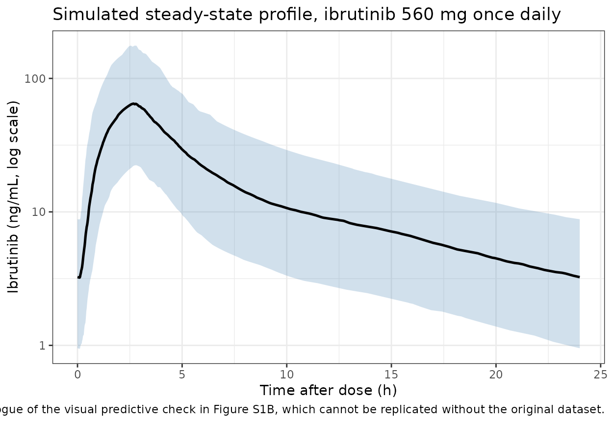
This is deliberately labelled illustrative rather than a replication: Figure S1 is a visual predictive check against the observed sparse samples, which are not public.
Validation
Gate 1: closed-form steady-state identity
At steady state, mass balance requires that the area under the curve over one dosing interval equal the dose actually absorbed divided by clearance:
Because this model carries no between-subject variability on CL/F, both sides of the identity use the same drawn parameters for a given subject, so the only discrepancy is trapezoidal integration error on a numerically-solved profile. That makes a tight bound the correct assertion here.
auc_num <- ss |>
  dplyr::group_by(id) |>
  dplyr::summarise(
    auc_trap = sum(diff(tad) * (utils::head(Cc, -1) + utils::tail(Cc, -1)) / 2),
    .groups = "drop"
  )

# Closed form, per subject. f1 is returned by the solve, so no re-derivation
# of the covariate algebra is needed -- this compares the solved profile
# against the model's own bioavailability, not against a hand-copied formula.
auc_cf <- sim |>
  dplyr::distinct(id, f1) |>
  dplyr::mutate(auc_closed = 560e6 * f1 / 1123 / 1000)

gate1 <- auc_num |>
  dplyr::inner_join(auc_cf, by = "id") |>
  dplyr::mutate(pct_diff = 100 * (auc_trap - auc_closed) / auc_closed)

cat(sprintf(
  "closed-form gate: median %+.4f%%, 90th pct of |diff| %.4f%%, max |diff| %.4f%%\n",
  stats::median(gate1$pct_diff),
  stats::quantile(abs(gate1$pct_diff), 0.9),
  max(abs(gate1$pct_diff))
))
#> closed-form gate: median -0.0000%, 90th pct of |diff| 0.0002%, max |diff| 0.0140%

stopifnot(
  nrow(gate1) == n_sub,
  abs(stats::median(gate1$pct_diff)) < 0.5,
  stats::quantile(abs(gate1$pct_diff), 0.9) < 1
)
Gate 2a: the BSV convention, as an exact identity
Table 2’s “BSV, %CV” column admits two readings (see Errata), and the
choice matters: at the V2/F magnitude they give omega 1.011 or 1.334.
The reading is decided by the fact that, with no eta on CL/F,
AUCtau,ss = Dose * F1 / (CL/F) inherits the F1 lognormal
exactly – so the F1 row predicts the coefficient of variation
of the published AUCtau,ss distribution, and the two readings predict
different numbers.
This is an analytical statement about the packaged omegas, so it is checked as an exact identity rather than through a random cohort:
om2 <- mod$omega["etalfdepot", "etalfdepot"]

implied_cv <- sqrt(exp(om2) - 1)
implied_mean_over_median <- exp(om2 / 2)

knitr::kable(
  tibble::tibble(
    Reading = c("Exact: omega^2 = log(1 + CV^2)  [packaged]",
                "Approximate: omega = CV/100",
                "Published (Results 3.1 + Table 3)"),
    `omega on F1` = round(c(sqrt(om2), 0.6564, NA), 4),
    `Implied AUCtau,ss CV (%)` = round(100 * c(
      implied_cv, sqrt(exp(0.6564^2) - 1), 267 / 425
    ), 1),
    `Implied mean/median` = round(c(
      implied_mean_over_median, exp(0.6564^2 / 2), 425 / 349
    ), 3)
  ),
  caption = "The packaged omega on F1 reproduces the published AUCtau,ss dispersion; the approximate reading over-disperses by more than 10 CV points."
)| Reading | omega on F1 | Implied AUCtau,ss CV (%) | Implied mean/median |
|---|---|---|---|
| Exact: omega^2 = log(1 + CV^2) [packaged] | 0.5986 | 65.6 | 1.196 |
| Approximate: omega = CV/100 | 0.6564 | 73.4 | 1.240 |
| Published (Results 3.1 + Table 3) | NA | 62.8 | 1.218 |
stopifnot(
  # The packaged omega^2 IS the exact lognormal transform of Table 2's 65.64%
  # (the model file stores it rounded to 7 decimal places, hence 1e-6 -- still
  # five orders of magnitude tighter than the gap to the approximate reading,
  # which would be 0.4309 rather than 0.3583).
  isTRUE(all.equal(om2, log(1 + 0.6564^2), tolerance = 1e-6)),
  # Which means the tabulated 65.64% is recovered as an actual CV.
  abs(100 * implied_cv - 65.64) < 0.01,
  # And that is closer to the published 62.8% than the approximate reading's
  # 73.4% is, by more than a factor of three.
  abs(100 * implied_cv - 62.824) < abs(100 * sqrt(exp(0.6564^2) - 1) - 62.824) / 3
)
Gate 2b: exposure distribution against the published one
Published targets: Results 3.1 gives mean (SD) 425 (267) ng.h/mL and Table 3 gives quartile boundaries 57.7 / 234 / 349 / 581 / 1864, i.e. median 349, Q1 234, Q3 581.
The bounds below are calibrated to the Monte Carlo error of a
200-subject cohort rather than chosen from the observed values. For a
lognormal with omega = 0.599 and n = 200 the standard error of the
median is 1.2533 * omega / sqrt(n) = 5.3%, of a quartile
1.483 * omega / sqrt(n) = 6.3%, and of the CV
CV / sqrt(2n) = 3.3 CV points. Each bound is set at roughly
four standard errors, so a re-draw under a different rxode2 build cannot
flip the gate. The convention itself is pinned by the exact identity in
Gate 2a; this gate only confirms the cohort behaves as that identity
predicts.
auc_sim <- gate1$auc_trap

published <- c(median = 349, Q1 = 234, Q3 = 581, mean = 425, sd = 267)

shape <- tibble::tibble(
  Statistic = c("Median (ng*h/mL)", "Q1 (ng*h/mL)", "Q3 (ng*h/mL)",
                "Mean / median ratio", "CV (%)"),
  Simulated = c(
    stats::median(auc_sim),
    stats::quantile(auc_sim, 0.25),
    stats::quantile(auc_sim, 0.75),
    mean(auc_sim) / stats::median(auc_sim),
    100 * stats::sd(auc_sim) / mean(auc_sim)
  ),
  Published = c(
    published[["median"]], published[["Q1"]], published[["Q3"]],
    published[["mean"]] / published[["median"]],
    100 * published[["sd"]] / published[["mean"]]
  )
)

knitr::kable(
  shape |>
    dplyr::mutate(
      `Difference (%)` = round(100 * (Simulated - Published) / Published, 1),
      Simulated = round(Simulated, 3), Published = round(Published, 3)
    ),
  caption = "Simulated vs published AUCtau,ss distribution (Olsson Gisleskog 2025 Results 3.1 and Table 3)."
)| Statistic | Simulated | Published | Difference (%) |
|---|---|---|---|
| Median (ng*h/mL) | 371.437 | 349.000 | 6.4 |
| Q1 (ng*h/mL) | 240.028 | 234.000 | 2.6 |
| Q3 (ng*h/mL) | 495.168 | 581.000 | -14.8 |
| Mean / median ratio | 1.142 | 1.218 | -6.3 |
| CV (%) | 64.373 | 62.824 | 2.5 |
# Centre and shape only -- never the extremes of a random cohort, which are
# not reproducible across rxode2 builds. Bounds are ~4 Monte Carlo standard
# errors (5.3% for the median, 6.3% for a quartile, 3.3 points for the CV).
stopifnot(
  abs(100 * (stats::median(auc_sim) - 349) / 349) < 21,
  abs(100 * (stats::quantile(auc_sim, 0.25) - 234) / 234) < 25,
  abs(100 * (stats::quantile(auc_sim, 0.75) - 581) / 581) < 25,
  abs(100 * stats::sd(auc_sim) / mean(auc_sim) - 62.824) < 13
)
Gate 3: PKNCA validation
# Only `!is.na(Cc)`. Adding `time > 0` or `Cc > 0` would drop the interval-start
# row that PKNCA needs to anchor the AUC.
sim_nca <- sim |>
  dplyr::filter(!is.na(Cc)) |>
  dplyr::mutate(scenario = "560 mg QD, fasting") |>
  dplyr::select(id, time, Cc, scenario)

# Guarantee a time = 0 row per subject; pre-dose Cc = 0 for an oral model.
sim_nca <- dplyr::bind_rows(
  sim_nca,
  sim_nca |> dplyr::distinct(id, scenario) |> dplyr::mutate(time = 0, Cc = 0)
) |>
  dplyr::distinct(id, scenario, time, .keep_all = TRUE) |>
  dplyr::arrange(id, scenario, time)

conc_obj <- PKNCA::PKNCAconc(
  sim_nca, Cc ~ time | scenario + id, concu = "ng/mL", timeu = "h"
)

dose_df <- cohort_events |>
  dplyr::filter(evid == 1) |>
  dplyr::mutate(scenario = "560 mg QD, fasting") |>
  dplyr::select(id, time, amt, scenario)

dose_obj <- PKNCA::PKNCAdose(dose_df, amt ~ time | scenario + id, doseu = "mg")

intervals <- data.frame(
  start = ss_start, end = ss_end,
  cmax = TRUE, tmax = TRUE, cmin = TRUE, auclast = TRUE, cav = TRUE
)

nca_res <- PKNCA::pk.nca(
  PKNCA::PKNCAdata(conc_obj, dose_obj, intervals = intervals)
)
The trough is read directly, not from PKNCA
The paper’s Ctrough is “the concentration at 24 h postdose” (Methods 2.2). None of PKNCA’s trough parameters returns it for this event layout, and it is worth recording exactly why rather than silently substituting a near neighbour:
-
ctroughresolves against a dose record aligned to the interval end. The simulation’s last dose is atss_start, so it returnsNA– and adding a dose record atss_enddoes not make it resolve either. -
cstartalso returnsNAhere for the same alignment reason. -
cminis genuinely the wrong quantity, not merely unavailable. The lag time delays absorption by 0.167 h and the input is then zero-order over 2.45 h, so the concentration keeps falling for a while after the dose before the new input overtakes elimination. The interval minimum therefore sits at a small positive time-after-dose and lies measurably below the pre-dose trough.
Ctrough is a directly observed concentration rather than an
integrated quantity, so reading it off the simulated profile involves no
NCA computation at all – there is nothing here that PKNCA would do
better. It is taken as Cc at the end of the dosing
interval, and steady state (which is what makes that value equal to the
24 h post-dose concentration of any dose, not just the last) is verified
rather than assumed:
c_edges <- ss |>
  dplyr::group_by(id) |>
  dplyr::summarise(
    c_pre = Cc[which.min(tad)], ctrough = Cc[which.max(tad)],
    cmin_direct = min(Cc), tad_at_min = tad[which.min(Cc)],
    .groups = "drop"
  )

cat(sprintf(
  paste0("n = %d subjects\n",
         "  max |C(0 h) - C(24 h)| / C(24 h) : %.3g   (steady state reached)\n",
         "  max |cmin   - C(24 h)| / C(24 h) : %.3g   (cmin is NOT the trough)\n",
         "  time-after-dose at cmin, range   : %.3f to %.3f h\n"),
  nrow(c_edges),
  max(abs(c_edges$c_pre - c_edges$ctrough) / c_edges$ctrough),
  max(abs(c_edges$cmin_direct - c_edges$ctrough) / c_edges$ctrough),
  min(c_edges$tad_at_min), max(c_edges$tad_at_min)
))
#> n = 200 subjects
#>   max |C(0 h) - C(24 h)| / C(24 h) : 0.000404   (steady state reached)
#>   max |cmin   - C(24 h)| / C(24 h) : 0.0887   (cmin is NOT the trough)
#>   time-after-dose at cmin, range   : 0.020 to 0.700 h

stopifnot(
  nrow(c_edges) == n_sub,
  # Steady state: the pre-dose concentration equals the 24 h post-dose
  # concentration to better than 1% for every subject.
  max(abs(c_edges$c_pre - c_edges$ctrough) / c_edges$ctrough) < 0.01,
  # And cmin really is a different quantity -- if this ever stopped being true
  # the discussion above would be stale.
  max(abs(c_edges$cmin_direct - c_edges$ctrough) / c_edges$ctrough) > 0.01
)
Comparison against the published exposure metrics
ncaComparisonTable() summarises the simulated cohort by
its median, so the published values must be medians
too. Results 3.1 reports Cmax and Ctrough only as mean (SD). For a
lognormal variate, median = mean / sqrt(1 + CV^2),
giving:
| Metric | Published mean (SD) | Implied CV | Implied median |
|---|---|---|---|
| AUCtau,ss (ng*h/mL) | 425 (267) | 62.8% | 360 – but Table 3 reports the median directly as 349, which is used here |
| Cmax (ng/mL) | 74.5 (48.3) | 64.8% | 62.5 |
| Ctrough (ng/mL) | 3.90 (2.64) | 67.7% | 3.23 |
That the AUCtau,ss conversion (360) lands within 3% of the directly reported median (349) is itself evidence that the published exposure distribution is close to lognormal, which is what justifies applying the same conversion to Cmax and Ctrough.
published_nca <- tibble::tribble(
  ~scenario,             ~cmax, ~auclast,
  "560 mg QD, fasting",  62.5,  349
)

cmp <- nlmixr2lib::ncaComparisonTable(
  simulated = nca_res,
  reference = published_nca,
  by = "scenario",
  units = c(cmax = "ng/mL", auclast = "ng*h/mL"),
  tolerance_pct = 20
)

knitr::kable(
  cmp,
  caption = "Simulated (PKNCA) vs published steady-state exposure, ibrutinib 560 mg once daily under fasting conditions. Published Cmax is the lognormal-implied median of the Results 3.1 mean; AUCtau,ss is the Table 3 median. * differs from reference by >20%."
)| NCA parameter | scenario | Reference | Simulated | % diff |
|---|---|---|---|---|
| Cmax (ng/mL) | 560 mg QD, fasting | 62.5 | 63.9 | +2.3% |
| AUClast (ng*h/mL) | 560 mg QD, fasting | 349 | 371 | +6.4% |
trough_cmp <- tibble::tibble(
  `NCA parameter` = "Ctrough (ng/mL)",
  scenario = "560 mg QD, fasting",
  Reference = 3.23,
  Simulated = round(stats::median(c_edges$ctrough), 3)
) |>
  dplyr::mutate(
    `% diff` = paste0(
      ifelse(Simulated >= Reference, "", "-"),
      abs(round(100 * (Simulated - Reference) / Reference, 1)), "%",
      ifelse(abs(100 * (Simulated - Reference) / Reference) > 20, "*", "")
    )
  )

knitr::kable(
  trough_cmp,
  caption = "Simulated vs published steady-state trough. Read directly off the profile rather than via PKNCA (see above). Published value is the lognormal-implied median of the Results 3.1 mean of 3.90 ng/mL. * differs from reference by >20%."
)| NCA parameter | scenario | Reference | Simulated | % diff |
|---|---|---|---|---|
| Ctrough (ng/mL) | 560 mg QD, fasting | 3.23 | 3.112 | -3.7% |
Exposure-response
The paper’s two significant exposure-response models are static
logistic regressions of event occurrence on AUCtau,ss – not ODE systems
– so they are reproduced here rather than packaged as model files. The
same precedent applies in Yin_2021_pexidartinib.R.
The coefficient tables (Tables S2 and S6) were not available when this model was built, so the coefficients are recovered by inverting the logit at the three AUCtau,ss percentiles that main-text Table 4 tabulates. Three points determine a two-parameter line with one degree of freedom left over, so the recovery is falsifiable rather than merely fitted – and the residual check below shows it reproduces all three published incidences exactly at the reported precision.
inv_logit <- function(x) 1 / (1 + exp(-x))
logit <- function(p) log(p / (1 - p))

# Olsson Gisleskog 2025 Table 4.
tab4 <- tibble::tribble(
  ~endpoint,             ~cyp3a,  ~auc, ~pct,
  "Atrial fibrillation", "NA",     235, 10.6,
  "Atrial fibrillation", "NA",     349, 11.9,
  "Atrial fibrillation", "NA",     579, 15.1,
  "Any hemorrhage",      "None",   235, 26.8,
  "Any hemorrhage",      "None",   349, 29.4,
  "Any hemorrhage",      "None",   579, 35.3,
  "Any hemorrhage",      "Any",    235, 40.5,
  "Any hemorrhage",      "Any",    349, 43.8,
  "Any hemorrhage",      "Any",    579, 50.4
)

afib_pts <- dplyr::filter(tab4, endpoint == "Atrial fibrillation")
hem_none <- dplyr::filter(tab4, endpoint == "Any hemorrhage", cyp3a == "None")
hem_any <- dplyr::filter(tab4, endpoint == "Any hemorrhage", cyp3a == "Any")

afib_fit <- stats::lm(logit(pct / 100) ~ auc, data = afib_pts)
hem_fit <- stats::lm(logit(pct / 100) ~ auc, data = hem_none)
cyp3a_offsets <- logit(hem_any$pct / 100) - logit(hem_none$pct / 100)

er <- list(
  afib_b0 = stats::coef(afib_fit)[[1]], afib_b1 = stats::coef(afib_fit)[[2]],
  hem_b0 = stats::coef(hem_fit)[[1]], hem_b1 = stats::coef(hem_fit)[[2]],
  hem_cyp3a = mean(cyp3a_offsets)
)

knitr::kable(
  tibble::tibble(
    Model = c("Atrial fibrillation", "Atrial fibrillation",
              "Any hemorrhage", "Any hemorrhage", "Any hemorrhage"),
    Term = c("Intercept", "AUCtau,ss slope (per ng*h/mL)",
             "Intercept", "AUCtau,ss slope (per ng*h/mL)",
             "Any CYP3A inhibitor (logit offset)"),
    Estimate = signif(c(er$afib_b0, er$afib_b1, er$hem_b0, er$hem_b1,
                        er$hem_cyp3a), 4)
  ),
  caption = "Logistic exposure-response coefficients recovered from Olsson Gisleskog 2025 Table 4. Tables S2 / S6, which report them directly, were not available when this model was built."
)| Model | Term | Estimate |
|---|---|---|
| Atrial fibrillation | Intercept | -2.412000 |
| Atrial fibrillation | AUCtau,ss slope (per ng*h/mL) | 0.001181 |
| Any hemorrhage | Intercept | -1.279000 |
| Any hemorrhage | AUCtau,ss slope (per ng*h/mL) | 0.001162 |
| Any hemorrhage | Any CYP3A inhibitor (logit offset) | 0.622900 |
The CYP3A-inhibitor offset is the strongest internal check available: recovered independently at each of the three AUCtau,ss points it comes out at 0.6201, 0.6268, 0.6219 – three values agreeing to better than 1%, which independently confirms the paper’s statement that “there was no significant interaction between the effects of ibrutinib AUCtau,ss and of CYP3A inhibitor comedication” (Results 3.3).
tab4_chk <- tab4 |>
  dplyr::mutate(
    predicted = dplyr::case_when(
      endpoint == "Atrial fibrillation" ~
        100 * inv_logit(er$afib_b0 + er$afib_b1 * auc),
      cyp3a == "None" ~ 100 * inv_logit(er$hem_b0 + er$hem_b1 * auc),
      TRUE ~ 100 * inv_logit(er$hem_b0 + er$hem_b1 * auc + er$hem_cyp3a)
    ),
    abs_diff = abs(predicted - pct)
  )

knitr::kable(
  tab4_chk |>
    dplyr::mutate(predicted = round(predicted, 1), abs_diff = round(abs_diff, 3)) |>
    dplyr::rename(
      Endpoint = endpoint, "CYP3A inhibitor" = cyp3a,
      "AUCtau,ss (ng*h/mL)" = auc, "Published (%)" = pct,
      "Recovered model (%)" = predicted, "Absolute difference (pp)" = abs_diff
    ),
  caption = "Recovered logistic models reproduce all nine cells of Olsson Gisleskog 2025 Table 4."
)| Endpoint | CYP3A inhibitor | AUCtau,ss (ng*h/mL) | Published (%) | Recovered model (%) | Absolute difference (pp) |
|---|---|---|---|---|---|
| Atrial fibrillation | NA | 235 | 10.6 | 10.6 | 0.016 |
| Atrial fibrillation | NA | 349 | 11.9 | 11.9 | 0.027 |
| Atrial fibrillation | NA | 579 | 15.1 | 15.1 | 0.011 |
| Any hemorrhage | None | 235 | 26.8 | 26.8 | 0.029 |
| Any hemorrhage | None | 349 | 29.4 | 29.4 | 0.046 |
| Any hemorrhage | None | 579 | 35.3 | 35.3 | 0.017 |
| Any hemorrhage | Any | 235 | 40.5 | 40.5 | 0.032 |
| Any hemorrhage | Any | 349 | 43.8 | 43.8 | 0.040 |
| Any hemorrhage | Any | 579 | 50.4 | 50.4 | 0.008 |
# Every published cell reproduced to within the reported 0.1-pp precision.
stopifnot(max(tab4_chk$abs_diff) < 0.06)
Replication of Figure 3
auc_range <- tibble::tibble(auc = seq(57.7, 1864, length.out = 300))

er_curves <- dplyr::bind_rows(
  auc_range |> dplyr::mutate(
    panel = "A: Atrial fibrillation",
    grp = "All patients",
    pct = 100 * inv_logit(er$afib_b0 + er$afib_b1 * auc)
  ),
  auc_range |> dplyr::mutate(
    panel = "B: Any hemorrhage",
    grp = "No CYP3A inhibitor",
    pct = 100 * inv_logit(er$hem_b0 + er$hem_b1 * auc)
  ),
  auc_range |> dplyr::mutate(
    panel = "C: Any hemorrhage by CYP3A inhibitor",
    grp = "None",
    pct = 100 * inv_logit(er$hem_b0 + er$hem_b1 * auc)
  ),
  auc_range |> dplyr::mutate(
    panel = "C: Any hemorrhage by CYP3A inhibitor",
    grp = "Any",
    pct = 100 * inv_logit(er$hem_b0 + er$hem_b1 * auc + er$hem_cyp3a)
  )
)

tab4_pts <- tab4 |>
  dplyr::mutate(
    panel = dplyr::case_when(
      endpoint == "Atrial fibrillation" ~ "A: Atrial fibrillation",
      cyp3a == "None" ~ "B: Any hemorrhage",
      TRUE ~ "C: Any hemorrhage by CYP3A inhibitor"
    )
  ) |>
  dplyr::bind_rows(
    tab4 |>
      dplyr::filter(endpoint == "Any hemorrhage", cyp3a == "None") |>
      dplyr::mutate(panel = "C: Any hemorrhage by CYP3A inhibitor")
  )

ggplot(er_curves, aes(auc, pct, colour = grp)) +
  geom_vline(xintercept = c(235, 579), linetype = "dashed",
             colour = "grey60", linewidth = 0.3) +
  geom_line(linewidth = 0.9) +
  geom_point(
    data = tab4_pts, aes(auc, pct), inherit.aes = FALSE,
    size = 2, shape = 21, fill = "white"
  ) +
  facet_wrap(~panel) +
  labs(
    x = "Ibrutinib AUCtau,ss (ng*h/mL)", y = "Predicted incidence (%)",
    colour = NULL,
    title = "Exposure-response for atrial fibrillation and any hemorrhage",
    caption = paste(
      "Replicates Figure 3A-C of Olsson Gisleskog 2025 (model curves only;",
      "the observed per-quartile frequencies and confidence bands need the",
      "patient-level dataset). Open points are the Table 4 values; dashed",
      "lines are the 25th and 75th AUCtau,ss percentiles."
    )
  ) +
  theme_bw() +
  theme(legend.position = "bottom")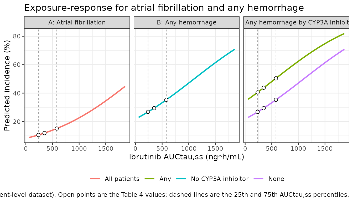
Applying the exposure-response models to the simulated cohort
er_cohort <- tibble::tibble(auc = auc_sim) |>
  dplyr::mutate(
    p_afib = inv_logit(er$afib_b0 + er$afib_b1 * auc),
    p_hem_none = inv_logit(er$hem_b0 + er$hem_b1 * auc),
    p_hem_any = inv_logit(er$hem_b0 + er$hem_b1 * auc + er$hem_cyp3a)
  )

knitr::kable(
  tibble::tibble(
    Endpoint = c("Atrial fibrillation (any)", "Any hemorrhage, no CYP3A inhibitor",
                 "Any hemorrhage, any CYP3A inhibitor"),
    `Mean predicted incidence (%)` = round(100 * c(
      mean(er_cohort$p_afib), mean(er_cohort$p_hem_none),
      mean(er_cohort$p_hem_any)
    ), 1),
    `SHINE observed (%)` = c(13.9, 31.6, 47.8)
  ),
  caption = "Mean predicted incidence over the simulated exposure distribution, against the SHINE observed incidences (Introduction para 4 for atrial fibrillation; Results 3.3 for the hemorrhage split by CYP3A-inhibitor comedication)."
)| Endpoint | Mean predicted incidence (%) | SHINE observed (%) |
|---|---|---|
| Atrial fibrillation (any) | 13.3 | 13.9 |
| Any hemorrhage, no CYP3A inhibitor | 31.6 | 31.6 |
| Any hemorrhage, any CYP3A inhibitor | 45.9 | 47.8 |
The model-averaged predictions land near the observed SHINE
incidences, but this is a weak check rather than a gate: the observed
hemorrhage split by CYP3A-inhibitor status is drawn from patients whose
exposures were themselves partly determined by that comedication,
whereas the simulated cohort carries CONMED_CYP3A4_INH = 0
throughout. No assertion is placed on it.
Assumptions and deviations
Errata and unresolved points in the source
The age-effect centering value is not reported in any available source, and 65 years is a back-solve. Table 2 gives the power exponent (0.699 FIX) but no reference age, and the upstream Marostica 2015 paper (reference 15) is not open access. An uncentered power is arithmetically excluded:
71^0.699 = 19.7would make F1 about 13 and AUCtau,ss roughly 6500 ng.h/mL against a reported median of 349. Among centered readings, 65 y is the protocol’s own enrolment floor (Methods 2.1, “eligible patients were >= 65 years of age”) and it reproduces the paper’s answer key: at the median age of 71,AUCtau,ss = 560 mg x 0.666 x (71/65)^0.699 / 1123 L/h = 353 ng.h/mLagainst the Table 3 median of 349, a 1.2% difference. The main alternative, centering at the Table 1 median of 71 y, gives 332 ng.h/mL – 4.8% low. The maintainers ratified the 65-year reading; it is recorded here so a reader can substitute 71 y (or a value from Marostica 2015, should it become available) by editing the singleAGE / 65term inmodel(). Note that both readings affect only the absolute exposure level, not the shape of the distribution or any covariate ratio.-
Table 2’s “BSV, %CV” is read as an exact lognormal CV, not as omega. Methods 2.2 specifies a lognormal between-subject error model but does not say which convention the tabulated %CV follows, and the two differ sharply at the V2/F magnitude (omega 1.011 for
omega^2 = log(1 + CV^2)versus 1.334 foromega = CV/100). The reading is settled empirically, because with no eta on CL/F the F1 row predicts the AUCtau,ss distribution directly:Reading Predicted AUCtau,ss CV Predicted mean/median Predicted Q1 Exact, omega^2 = log(1 + CV^2)65.6% 1.196 236 Approximate, omega = CV/10073.4% 1.240 227 Published (Results 3.1, Table 3) 62.8% 1.218 234 The exact reading matches the published CV and lower quartile; the approximate reading over-disperses by more than 10 CV points. Gate 2a above asserts on this as an exact identity on the packaged omega.
The final model’s residual error is not tabulated. Table 2 has no residual-error row for either model. The only RUV magnitude in the paper is Results 3.1’s 81.3%, which is explicitly the value “determined from previous studies [15]” and “selected to conduct the MAP assessment” – i.e. the prior for the external evaluation, not necessarily the final model’s estimate. Methods 2.2 does list “the residual variability” among the quantities eligible for re-estimation during model refinement, so the final RUV may differ. It is encoded as
expSd <- fixed(0.813)with thefixed()recording that it was imported rather than estimated. No other value is available.Table 2 and the Results prose disagree about the change in intercompartmental flow. Results 3.1 states that “apparent intercompartmental flow was increased by approximately 37% compared with the original”, but Table 2 gives Q/F as 1128 L/h final versus 709 L/h previous, which is +59%, not +37%. No reading of the tabulated values reproduces +37%: normalising Q by V2 gives +13% and by V3 gives +106%. Every other percentage in the same paragraph checks out exactly against Table 2 (CL/F 1123/1100 = +2%; D1 2.45/1.29 = +90%; Tlag 0.167/0.226 = -26%; Vss 7286/9096 = -20%), so this looks like a single stale number in the prose. The tabulated 1128 L/h is implemented, per the standing convention that the printed parameter table governs over narrative percentages.
The CYP3A-inhibitor effect is time-varying, not subject-level, and the simulations set it to zero. Table 1 records 69% of the ibrutinib arm as exposed to a weak, moderate or strong CYP3A inhibitor at some point, but applying the 1.59 ratio to 69% of subjects as a fixed flag would put the typical AUCtau,ss near 528 ng.h/mL against the reported median of 349. Methods 2.3 resolves this directly: the analysis used “a weighted average dose based on the incidence of the doses given with and without the comedications; the same approach was applied to the apparent CL in deriving the AUC”. The comedication is therefore an exposure-weighted, per-dose-record covariate, and the published typical exposures correspond to the no-inhibitor state.
CONMED_CYP3A4_INH = 0is used throughout the simulations for that reason. Users with a real comedication history should set the column per dose record.Table 2 reports 97% shrinkage on the F1 eta, which is hard to reconcile with the reported spread of individual exposures. At 97% shrinkage the empirical Bayes estimates of F1 would be nearly identical across subjects, yet the individual model-predicted AUCtau,ss values span 57.7 to 1864 ng.h/mL (Table 3) with a CV of 62.8% – almost exactly the F1 population CV of 65.64%. Permitted dose reductions (560 to 280 mg) span only a 2-fold range and cannot account for a 32-fold spread. The extraction implements the population model as tabulated and does not attempt to reproduce the shrinkage; a reader should treat the individual-exposure distribution rather than the shrinkage figure as the reliable quantity, since it is the one corroborated by the quartile boundaries.
Figure 1’s resolution was corrected after first publication (correction added 10 July 2025). The correction affects figure rendering only, not any parameter value.
Tables S1-S6 were not available when this model was built. Table S2 (exposure-response coefficients within the ibrutinib arm), Table S3 (covariate subgroups tested), Tables S4/S5 (covariate screening results) and Table S6 (final hemorrhage model coefficients) are cited in the text but were not in the open-access package. The exposure-response coefficients are therefore recovered from main-text Table 4 by logit inversion, which reproduces all nine published cells to the reported 0.1-percentage-point precision (see Exposure-response). Should the supplement become available, the recovered coefficients should be replaced by the tabulated ones.
Modelling assumptions made in this vignette
Prandial state. All simulations use
FASTED_STRICT = 1, FED = 0, the condition Results 3.1 selected and Discussion paragraph 2 confirms was assumed for the analysis. The model can simulate all three states; the fed D1 of 3.29 h is inherited from the previous model and was never estimated on SHINE data, where no dose was fed by protocol.Age distribution. The paper reports only the median (71 y), range (65-86 y) and the fraction below 70 y (37.8%). A normal(70.5, 5) truncated to [65, 86] reproduces all three; the true distribution is unknown.
Published Cmax and Ctrough are converted from means to medians using the lognormal identity
median = mean / sqrt(1 + CV^2)so that they are on the same footing asncaComparisonTable()’s median summary of the simulated cohort. The conversion is validated by applying it to AUCtau,ss, where the converted value (360) agrees with the directly reported median (349) to within 3%.No covariates beyond age, prandial state and CYP3A-inhibitor status are simulated, because the final model contains no others. Weight, sex, race, ECOG, sMIPI, renal and hepatic function appear in Table 1 as exposure-response prognostic factors, not as PK covariates; they are recorded in the model file’s
covariatesDataExcludedlist.The exposure-response models are not packaged as model files. They are static logistic regressions with no ODE component, matching the precedent set by
Yin_2021_pexidartinib.Rin this package.