Vedolizumab (Hanzel 2022)
Source:vignettes/articles/Hanzel_2022_vedolizumab.Rmd
Hanzel_2022_vedolizumab.RmdModel and source
- Citation: Hanzel J, Dreesen E, Vermeire S, Lowenberg M, Hoentjen F, Bossuyt P, Clasquin E, Baert FJ, D’Haens GR, Mathot R. Pharmacokinetic-Pharmacodynamic Model of Vedolizumab for Targeting Endoscopic Remission in Patients With Crohn Disease: Posthoc Analysis of the LOVE-CD Study. Inflamm Bowel Dis. 2022;28:689-699. doi:10.1093/ibd/izab143 (PMC9071095). A corrigendum (doi:10.1093/ibd/izab270; PMC9071094) corrects reference 36 only and does not change any parameter value.
- Description: Two-compartment population PK model for vedolizumab (humanised anti-alpha4-beta7 integrin IgG1 monoclonal antibody) with parallel linear and Michaelis-Menten elimination in adults with active Crohn’s disease (LOVE-CD trial), with interindividual and inter-occasion variability (induction / maintenance) on linear clearance and time-varying effects of serum albumin, antibodies to vedolizumab and anti-TNF-naive status on linear clearance, plus the sequential first-order discrete-time Markov model for endoscopic remission (SES-CD < 4) and dropout at weeks 26 and 52 driven by the individual predicted week-22 trough concentration (Hanzel 2022). Q, Vp, Km and Vmax were held at the Rosario 2015 values.
- Article: https://doi.org/10.1093/ibd/izab143 (open access, PMC9071095)
- Corrigendum: https://doi.org/10.1093/ibd/izab270 (PMC9071094; corrects reference 36 only, no parameter values affected)
Hanzel et al. analysed the first 110 patients of LOVE-CD, a phase 4 open-label trial of intravenous vedolizumab in active Crohn’s disease. The paper has two sequentially fitted parts, both packaged in the single model file:
- A population PK model: two compartments with
parallel linear and Michaelis-Menten elimination. The peripheral volume,
intercompartmental clearance, Km and Vmax were held at the Rosario 2015
values (see
modellib("Rosario_2015_vedolizumab")). Linear clearance carries interindividual and inter-occasion variability and time-varying covariate effects of serum albumin, antibodies to vedolizumab and anti-TNF-naive status. - A first-order discrete-time Markov model for
endoscopic remission (SES-CD < 4) at weeks 26 and 52. States are no
remission (0), remission (1) and dropout (2). The exposure driver is the
individual predicted vedolizumab concentration at week 22
(
IPRED22), the trough before the week-22 infusion.
Population
The PK analysis included 108 of 110 LOVE-CD patients with at least one quantifiable vedolizumab sample (Hanzel 2022 Table 1). In total, 737 serum samples were drawn, all before an infusion. Of the 108 patients, 69% were women. Median age was 36 years (IQR 28-46), median weight 71 kg (IQR 61-82) and median baseline albumin 41 g/L (IQR 38-43). Baseline CDAI was 261 (IQR 238-312) and baseline SES-CD 12 (IQR 7-17). Previous exposure to anti-TNF agents was very common (89%). Antibodies to vedolizumab were detected in 4 patients (3.7%), on 10 samples.
Vedolizumab 300 mg was infused at weeks 0, 2 and 6 and every 8 weeks thereafter through week 52. An extra week-10 infusion was given to the 68 patients (63%) whose CDAI had not fallen by at least 70 points. Endoscopic remission was seen in 36 patients (33%) at week 26 and 40 (37%) at week 52. The trial ran at sites in the Netherlands and Belgium.
The same information is available programmatically:
str(readModelDb("Hanzel_2022_vedolizumab")()$population)
#> Warning: some etas defaulted to non-mu referenced, possible parsing error: etaiov_cl_1, etaiov_cl_2
#> as a work-around try putting the mu-referenced expression on a simple line
#> List of 13
#>  $ species         : chr "human"
#>  $ n_subjects      : int 108
#>  $ n_studies       : int 1
#>  $ age_median      : chr "36 years (IQR 28-46)"
#>  $ weight_median   : chr "71 kg (IQR 61-82)"
#>  $ sex_female_pct  : num 69
#>  $ disease_state   : chr "Active Crohn's disease (CDAI > 220 with mucosal ulceration at baseline ileocolonoscopy); baseline CDAI median 2"| __truncated__
#>  $ dose_range      : chr "Vedolizumab 300 mg IV at weeks 0, 2 and 6 and every 8 weeks thereafter through week 52; 68 patients (63%) recei"| __truncated__
#>  $ regions         : chr "Netherlands, Belgium"
#>  $ prior_tnf_pct   : num 89
#>  $ albumin_median  : chr "41 g/L (IQR 38-43)"
#>  $ ada_positive_pct: num 3.7
#>  $ notes           : chr "LOVE-CD (NCT02646683), a phase 4 prospective open-label multicentre trial. 108 of 110 enrolled patients had at "| __truncated__
Source trace
Every ini() value carries an in-file comment pointing at
its source. The table below collects them in one place.
| Equation / parameter | Value | Source location |
|---|---|---|
lcl (CL_L) |
log(0.215) L/day | Table 2, final model |
lvc (V1) |
log(4.92) L | Table 2, final model |
lvp (V2) |
log(1.65) L, held constant | Table 2 (‘FIX’, from Rosario 2015) |
lq (Q) |
log(0.12) L/day, held constant | Table 2 (‘FIX’, from Rosario 2015) |
lkm (Km) |
log(0.964) mg/L, held constant | Table 2 (‘FIX’, from Rosario 2015) |
lvmax (Vm) |
log(0.265) mg/day, held constant | Table 2 (‘FIX’, from Rosario 2015) |
e_alb_cl |
-0.020 per g/L | Table 2; Equation 1; Appendix THETA(9)
|
e_ada_cl |
1.89 | Table 2; Appendix THETA(11)
|
e_tnfnaive_cl |
0.755 | Table 2; Appendix THETA(10)
|
etalcl |
0.262^2 = 0.068644 | Table 2 IIV CL_L 26.2 CV% (footnote: CV = sqrt(variance)) |
etalvc |
0, held constant | Appendix ETA(2) on V1; variance not reported (see
Assumptions) |
etaiov_cl_1, etaiov_cl_2
|
0.152^2 = 0.023104 | Table 2 IOV CL_L 15.2 CV%; Appendix
$OMEGA BLOCK(1) SAME
|
addSd |
0.469 mg/L | Table 2 additive error |
propSd |
0.189 | Table 2 proportional error; Appendix $ERROR
W
|
emax_01 |
0.7, held constant | Table 2 (70% FIX); Appendix THETA(1)
|
lec50_01 |
log(20.0) mg/L | Table 2, final model |
emax_02 |
1, held constant | Table 2; Appendix THETA(3)
|
let50_02 |
log(515) days | Table 2, final model |
emax_10, lec50_10
|
1 (held constant), log(1.78) mg/L | Table 2, final model |
emax_12, lec50_12
|
1 (held constant), log(0.47) mg/L | Table 2, final model |
| CL_L covariate model | CL = TVCL * (1 + (ALB - 41) * th9) * th10^TNFNAIVE * th11^ADA * exp(eta1 + IOV) |
Equation 1; Appendix $PK
|
| ODEs | linear + Michaelis-Menten elimination from central | Appendix $DES; Supplementary Figure 1 |
p01, p02
|
EMAX01 * C22 / (EC50 + C22),
EMAX02 * DAYS / (ET50 + DAYS)
|
Appendix $PRED; Supplementary Figure 1 |
DAYS |
VISIT * 7 + 0.01 |
Appendix $PRED
|
| Transition fractions |
P(0->2) = P02 (1 - P01),
P(1->2) = P12 (1 - P10)
|
Appendix $PRED
|
p10, p12
|
EC50 / (EC50 + C22) (inhibitory, Emax = 1) |
Table 2 final; form inferred (see Assumptions) |
Closed-form checks of the reported effects
The paper quotes four effect sizes that follow directly from the parameters.
mod <- readModelDb("Hanzel_2022_vedolizumab")
ini_df <- rxode2::rxode(mod)$iniDf
#> ℹ parameter labels from comments will be replaced by 'label()'
#> Warning: some etas defaulted to non-mu referenced, possible parsing error: etaiov_cl_1, etaiov_cl_2
#> as a work-around try putting the mu-referenced expression on a simple line
th <- setNames(ini_df$est, ini_df$name)

checks <- tibble::tribble(
  ~quantity, ~paper, ~model,
  "CL_L increase, albumin 41 -> 28 g/L (%)", 26,
  100 * ((1 + (28 - 41) * th[["e_alb_cl"]]) - 1),
  "CL_L increase with antibodies to vedolizumab (%)", 89,
  100 * (th[["e_ada_cl"]] - 1),
  "P(remission at week 26) at C22 = 20.0 mg/L (%)", 35,
  100 * th[["emax_01"]] * 20 / (exp(th[["lec50_01"]]) + 20)
)
knitr::kable(checks, digits = 2,
caption = "Effect sizes quoted in the Hanzel 2022 Results.")| quantity | paper | model |
|---|---|---|
| CL_L increase, albumin 41 -> 28 g/L (%) | 26 | 26 |
| CL_L increase with antibodies to vedolizumab (%) | 89 | 89 |
| P(remission at week 26) at C22 = 20.0 mg/L (%) | 35 | 35 |
The Results text also says CL_L is “+ 25% compared to no prior exposure” in patients previously exposed to biologics. The model carries the estimated multiplier 0.755 for anti-TNF-naive patients, i.e. a 24.5% lower CL_L than in exposed patients. Equivalently, exposed patients have 1 / 0.755 = 1.32-fold the CL_L of naive patients. The rounded “25%” in the text is the first of these.
Virtual cohort
The original data are not public. The simulations below use virtual
patients whose covariates approximate Table 1. Albumin is drawn from a
normal distribution with the cohort median of 41 g/L and an SD of 3.7
g/L, which matches the reported IQR of 38-43 g/L, truncated to 25-52
g/L. Antibodies to vedolizumab are set absent, since they were found on
only 1.4% of samples. The occasion column follows the paper:
OCC = 1 (induction) before the week-14 infusion and
OCC = 2 (maintenance) from day 98 onward.
Each infusion is 300 mg over 30 minutes into
central.
inf_rate <- 300 / (30 / 1440) # 300 mg over 30 min, in mg/day

make_cohort <- function(n, dose_weeks, obs_days, prior_tnf, regimen,
                        id_offset = 0L) {
  ids <- id_offset + seq_len(n)
  alb <- pmin(pmax(stats::rnorm(n, 41, 3.7), 25), 52)
  doses <- expand.grid(id = ids, time = dose_weeks * 7) |>
    mutate(evid = 1L, amt = 300, rate = inf_rate)
  obs <- expand.grid(id = ids, time = obs_days) |>
    mutate(evid = 0L, amt = NA_real_, rate = NA_real_)
  bind_rows(doses, obs) |>
    mutate(
      cmt = "central",
      ALB = alb[id - id_offset],
      ADA_POS = 0L,
      PRIOR_TNF = prior_tnf,
      OCC = ifelse(time < 98, 1L, 2L),
      regimen = regimen,
      tnf = ifelse(prior_tnf == 1, "Anti-TNF-experienced", "Anti-TNF-naive")
    ) |>
    arrange(id, time, desc(evid))
}
Endoscopic remission at week 26 by dosing regimen (Table 3)
Table 3 of the paper simulates three regimens in anti-TNF-naive and anti-TNF-experienced patients. The week-26 remission probability depends only on the week-22 trough. The cohorts below are therefore solved to day 154, using only the doses given before the week-22 infusion; the week-22 dose itself cannot change the pre-dose trough. Each of the six arms has 200 patients.
rxode2::rxSetSeed(2022)
set.seed(2022)
regimens <- list(
  "300 mg at weeks 0, 2, 6, 14, 22" = c(0, 2, 6, 14),
  "300 mg at weeks 0, 2, 6, 10, 14, 22" = c(0, 2, 6, 10, 14),
  "300 mg at weeks 0, 2, 6, 10, 14, 18, 22" = c(0, 2, 6, 10, 14, 18)
)
n_arm <- 200L
arms <- expand.grid(regimen = names(regimens), prior_tnf = c(0L, 1L),
                    stringsAsFactors = FALSE)
events_t3 <- bind_rows(lapply(seq_len(nrow(arms)), function(i) {
  make_cohort(
    n = n_arm,
    dose_weeks = regimens[[arms$regimen[i]]],
    obs_days = seq(0, 154, by = 7),
    prior_tnf = arms$prior_tnf[i],
    regimen = arms$regimen[i],
    id_offset = (i - 1L) * n_arm
  )
}))
stopifnot(!anyDuplicated(unique(events_t3[, c("id", "time", "evid")])))

sim_t3 <- rxode2::rxSolve(mod, events = events_t3,
                          keep = c("regimen", "tnf"),
                          returnType = "data.frame")
#> ℹ parameter labels from comments will be replaced by 'label()'
#> Warning: some etas defaulted to non-mu referenced, possible parsing error: etaiov_cl_1, etaiov_cl_2
#> as a work-around try putting the mu-referenced expression on a simple line
#> ℹ omega/sigma items treated as zero: 'etalvc'
published_t3 <- tibble::tribble(
  ~regimen, ~tnf, ~paper,
  "300 mg at weeks 0, 2, 6, 14, 22", "Anti-TNF-naive", 29.1,
  "300 mg at weeks 0, 2, 6, 10, 14, 22", "Anti-TNF-naive", 33.9,
  "300 mg at weeks 0, 2, 6, 10, 14, 18, 22", "Anti-TNF-naive", 46.5,
  "300 mg at weeks 0, 2, 6, 14, 22", "Anti-TNF-experienced", 20.2,
  "300 mg at weeks 0, 2, 6, 10, 14, 22", "Anti-TNF-experienced", 24.2,
  "300 mg at weeks 0, 2, 6, 10, 14, 18, 22", "Anti-TNF-experienced", 40.0
)

t3 <- sim_t3 |>
  filter(time == 154) |>
  group_by(regimen, tnf) |>
  summarise(
    c22 = median(Cc),
    simulated = 100 * median(prob_endorem_wk26),
    .groups = "drop"
  ) |>
  inner_join(published_t3, by = c("regimen", "tnf")) |>
  mutate(diff = simulated - paper) |>
  arrange(tnf, simulated)

t3 |>
  rename(
    "Regimen" = regimen,
    "Group" = tnf,
    "Median C22 (mg/L)" = c22,
    "Simulated median P(remission), %" = simulated,
    "Hanzel 2022 Table 3, %" = paper,
    "Difference (points)" = diff
  ) |>
  knitr::kable(digits = 1, caption = paste(
    "Replicates Table 3 of Hanzel 2022: median predicted probability of",
    "endoscopic remission at week 26."
))| Regimen | Group | Median C22 (mg/L) | Simulated median P(remission), % | Hanzel 2022 Table 3, % | Difference (points) |
|---|---|---|---|---|---|
| 300 mg at weeks 0, 2, 6, 14, 22 | Anti-TNF-experienced | 8.4 | 20.6 | 20.2 | 0.4 |
| 300 mg at weeks 0, 2, 6, 10, 14, 22 | Anti-TNF-experienced | 10.8 | 24.6 | 24.2 | 0.4 |
| 300 mg at weeks 0, 2, 6, 10, 14, 18, 22 | Anti-TNF-experienced | 27.6 | 40.6 | 40.0 | 0.6 |
| 300 mg at weeks 0, 2, 6, 14, 22 | Anti-TNF-naive | 12.3 | 26.7 | 29.1 | -2.4 |
| 300 mg at weeks 0, 2, 6, 10, 14, 22 | Anti-TNF-naive | 20.6 | 35.5 | 33.9 | 1.6 |
| 300 mg at weeks 0, 2, 6, 10, 14, 18, 22 | Anti-TNF-naive | 41.9 | 47.4 | 46.5 | 0.9 |
The simulated medians reproduce Table 3 to within a few percentage points in all six cells, including the gain from shortening the interval to every 4 weeks. The checks are on the cohort median, which is stable across rxode2 builds, and on the direction of the regimen and anti-TNF effects. Those contrasts are many times larger than the Monte-Carlo error of a 200-patient median.
stopifnot(
  # Structural: a mis-transcribed EC50, CL or covariate effect moves these
  # medians by far more than 6 points.
  all(abs(t3$diff) < 6),
  # Every-4-weeks dosing beats per-label dosing in both groups.
  all(t3 |> group_by(tnf) |>
        summarise(gain = max(simulated) - min(simulated)) |>
        pull(gain) > 10)
)
Exposure-response curve (Figure 2)
Figure 2 of the paper overlays observed and predicted week-26 outcomes on quantiles of the week-22 concentration. Below are the model-predicted curves from the typical parameters: remission, dropout without remission, and persistent non-remission.
c22_grid <- c(seq(0.5, 80, by = 0.5))
p01 <- th[["emax_01"]] * c22_grid / (exp(th[["lec50_01"]]) + c22_grid)
days26 <- 26 * 7 + 0.01
p02 <- th[["emax_02"]] * days26 / (exp(th[["let50_02"]]) + days26)
er_curve <- tibble(
  C22 = c22_grid,
  `Endoscopic remission` = p01,
  `Dropout` = p02 * (1 - p01),
  `No remission` = 1 - p01 - p02 * (1 - p01)
) |>
  pivot_longer(-C22, names_to = "state", values_to = "prob")

ggplot(er_curve, aes(C22, 100 * prob, linetype = state)) +
  geom_line() +
  geom_point(data = tibble(C22 = 20, prob = 0.35), aes(C22, 100 * prob),
             inherit.aes = FALSE, colour = "red") +
  labs(x = "Individual predicted vedolizumab concentration at week 22 (mg/L)",
       y = "Probability at week 26 (%)", linetype = NULL,
       caption = paste("Model counterpart of Figure 2 of Hanzel 2022; red point:",
                       "35% at 20.0 mg/L quoted in the Results."))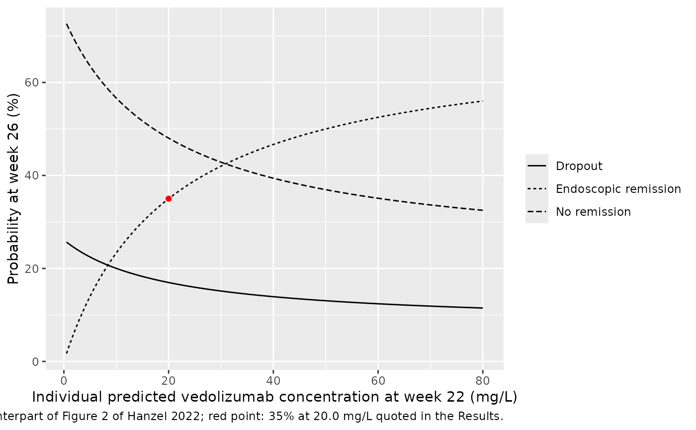
Week-52 Markov outcomes
The model also returns the marginal state probabilities at week 52. These come from chaining the baseline -> week 26 and week 26 -> week 52 transitions, all driven by the same week-22 concentration. The paper does not report simulated week-52 probabilities, so they cannot be checked against a published number. Two properties can be checked: the three state probabilities sum to 1 at each visit, and remission rises with exposure.
wk <- sim_t3 |>
  filter(time == 154) |>
  group_by(regimen, tnf) |>
  summarise(across(c(prob_endorem_wk26, prob_dropout_wk26,
                     prob_endorem_wk52, prob_dropout_wk52),
                   ~ 100 * median(.x)),
            .groups = "drop")
wk |>
  rename(
    "Regimen" = regimen, "Group" = tnf,
    "Remission wk 26, %" = prob_endorem_wk26,
    "Dropout wk 26, %" = prob_dropout_wk26,
    "Remission wk 52, %" = prob_endorem_wk52,
    "Dropout wk 52, %" = prob_dropout_wk52
  ) |>
knitr::kable(digits = 1, caption = "Median simulated state probabilities.")| Regimen | Group | Remission wk 26, % | Dropout wk 26, % | Remission wk 52, % | Dropout wk 52, % |
|---|---|---|---|---|---|
| 300 mg at weeks 0, 2, 6, 10, 14, 18, 22 | Anti-TNF-experienced | 40.6 | 15.5 | 55.3 | 27.0 |
| 300 mg at weeks 0, 2, 6, 10, 14, 18, 22 | Anti-TNF-naive | 47.4 | 13.7 | 63.3 | 22.7 |
| 300 mg at weeks 0, 2, 6, 10, 14, 22 | Anti-TNF-experienced | 24.6 | 19.7 | 33.9 | 38.0 |
| 300 mg at weeks 0, 2, 6, 10, 14, 22 | Anti-TNF-naive | 35.5 | 16.8 | 48.9 | 30.3 |
| 300 mg at weeks 0, 2, 6, 14, 22 | Anti-TNF-experienced | 20.6 | 20.7 | 28.2 | 40.9 |
| 300 mg at weeks 0, 2, 6, 14, 22 | Anti-TNF-naive | 26.7 | 19.1 | 37.0 | 36.4 |
at154 <- sim_t3 |> filter(time == 154)
stopifnot(
  max(abs(at154$prob_endorem_wk26 + at154$prob_dropout_wk26 +
            at154$prob_noendorem_wk26 - 1)) < 1e-10,
  max(abs(at154$prob_endorem_wk52 + at154$prob_dropout_wk52 +
            at154$prob_noendorem_wk52 - 1)) < 1e-10,
  cor(at154$Cc, at154$prob_endorem_wk52, method = "spearman") > 0.9
)
Trough concentrations over the LOVE-CD schedule (Figure 1)
Figure 1 of the paper is a prediction-corrected VPC of the trough samples. This section simulates the LOVE-CD schedule through week 52 with 200 patients. Infusions are at weeks 0, 2, 6, 14, 22, 30, 38 and 46, and 63% of patients get the extra week-10 infusion. Anti-TNF exposure is assigned at the trial rate of 89%. Troughs are read before each infusion and at week 52.
rxode2::rxSetSeed(1)
set.seed(1)
n_vpc <- 200L
trough_weeks <- c(2, 6, 10, 14, 22, 30, 38, 46, 52)
extra_wk10 <- stats::runif(n_vpc) < 0.63
prior <- as.integer(stats::runif(n_vpc) < 0.89)
events_vpc <- bind_rows(lapply(seq_len(n_vpc), function(i) {
  make_cohort(
    n = 1L,
    dose_weeks = c(0, 2, 6, if (extra_wk10[i]) 10, 14, 22, 30, 38, 46),
    obs_days = trough_weeks * 7 - 1e-4,
    prior_tnf = prior[i],
    regimen = "LOVE-CD",
    id_offset = i - 1L
  )
}))
sim_vpc <- rxode2::rxSolve(mod, events = events_vpc, returnType = "data.frame")
#> ℹ omega/sigma items treated as zero: 'etalvc'

vpc <- sim_vpc |>
  mutate(week = round(time / 7)) |>
  group_by(week) |>
  summarise(
    Q05 = quantile(Cc, 0.05), Q50 = median(Cc), Q95 = quantile(Cc, 0.95),
    .groups = "drop"
  )

ggplot(vpc, aes(week * 7, Q50)) +
  geom_ribbon(aes(ymin = Q05, ymax = Q95), alpha = 0.25) +
  geom_line() +
  geom_point() +
  labs(x = "Time (days)", y = "Simulated trough vedolizumab (mg/L)",
       caption = paste("Counterpart of Figure 1 of Hanzel 2022 (median and",
                       "5th-95th percentiles of simulated troughs)."))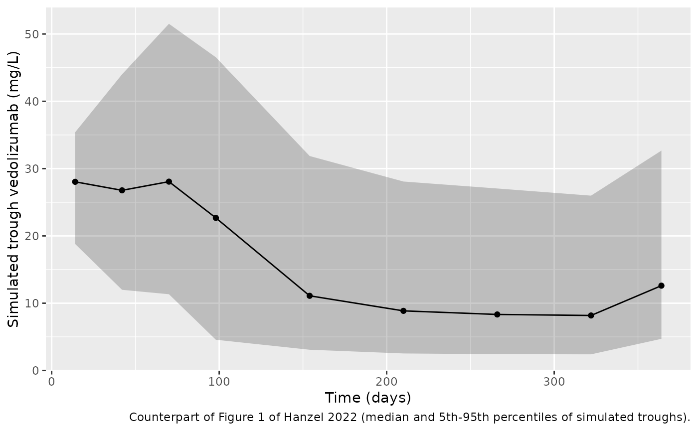
knitr::kable(vpc, digits = 1, caption = "Simulated trough percentiles by week.")| week | Q05 | Q50 | Q95 |
|---|---|---|---|
| 2 | 18.8 | 28.0 | 35.4 |
| 6 | 12.0 | 26.8 | 44.0 |
| 10 | 11.3 | 28.1 | 51.5 |
| 14 | 4.6 | 22.7 | 46.5 |
| 22 | 3.1 | 11.1 | 31.9 |
| 30 | 2.5 | 8.9 | 28.1 |
| 38 | 2.4 | 8.3 | 27.0 |
| 46 | 2.4 | 8.2 | 26.0 |
| 52 | 4.7 | 12.6 | 32.7 |
In Figure 1 of the paper, the observed median trough is roughly 25 mg/L during induction (days 14-98) and roughly 10-12 mg/L during maintenance. These values were read approximately from the plot. The simulated medians fall in the same ranges. Figure 1 is prediction-corrected, so only this broad agreement is checked.
PKNCA validation
The paper reports no NCA. For completeness, PKNCA is run over the first dosing interval (days 0-14) in typical-albumin patients, split by anti-TNF exposure. The anti-TNF-naive group should show the larger AUC, because its linear clearance is 0.755-fold that of the experienced group.
rxode2::rxSetSeed(7)
set.seed(7)
nca_obs <- sort(unique(c(0, 30 / 1440, 0.25, 0.5, 1, 2, 3, 5, 7, 10, 14)))
events_nca <- bind_rows(
  make_cohort(100L, 0, nca_obs, 1L, "first dose", id_offset = 0L),
  make_cohort(100L, 0, nca_obs, 0L, "first dose", id_offset = 100L)
)
sim_nca <- rxode2::rxSolve(mod, events = events_nca, keep = "tnf",
                           returnType = "data.frame") |>
  filter(!is.na(Cc)) |>
  select(id, time, Cc, tnf)
#> ℹ omega/sigma items treated as zero: 'etalvc'

conc_obj <- PKNCA::PKNCAconc(sim_nca, Cc ~ time | tnf + id)
dose_obj <- PKNCA::PKNCAdose(
  events_nca |> filter(evid == 1) |> select(id, time, amt, tnf),
  amt ~ time | tnf + id
)
intervals <- data.frame(start = 0, end = 14, cmax = TRUE, tmax = TRUE,
                        auclast = TRUE)
nca_res <- PKNCA::pk.nca(PKNCA::PKNCAdata(conc_obj, dose_obj,
                                          intervals = intervals))
nca_sum <- as.data.frame(nca_res$result) |>
  group_by(tnf, PPTESTCD) |>
  summarise(median = median(PPORRES), .groups = "drop") |>
  pivot_wider(names_from = PPTESTCD, values_from = median)
nca_sum |>
  rename("Group" = tnf, "Cmax (mg/L)" = cmax, "Tmax (day)" = tmax,
         "AUC0-14 (mg*day/L)" = auclast) |>
knitr::kable(digits = 2, caption = "First-dose NCA (medians, PKNCA).")| Group | AUC0-14 (mg*day/L) | Cmax (mg/L) | Tmax (day) |
|---|---|---|---|
| Anti-TNF-experienced | 574.21 | 60.93 | 0.02 |
| Anti-TNF-naive | 614.30 | 60.94 | 0.02 |
stopifnot(
  nca_sum$auclast[nca_sum$tnf == "Anti-TNF-naive"] >
    nca_sum$auclast[nca_sum$tnf == "Anti-TNF-experienced"]
)
Assumptions and deviations
-
Final-model form of the 1 -> 0 and 1 -> 2
transitions. The Appendix
$PREDcode models the transitions out of remission (P10,P12) as constant probabilities,THETA(5)andTHETA(6), bounded to (0, 1). Table 2’s final-model column instead listsEmax10 = 1 FIX,EC50,10 = 1.78 mg/L,Emax12 = 1 FIXandEC50,12 = 0.47 mg/L, with RSEs and bootstrap medians. The maintainers implemented the Table 2 parameterisation, for three reasons:- 1.78 lies outside the (0, 1) bound, so it cannot be a final value of the printed constant.
- With no random effects, the likelihood of the transitions out of
state 1 separates from the state-0 transitions. Had
P10andP12stayed constant, their final estimates would equal the base-model 10.0% and 2.8%. The paper reports different numbers with separate bootstrap results. - Only an inhibitory form,
P = EC50 / (EC50 + C22), is consistent with the estimates. At a typical week-22 trough of about 20 mg/L it gives about 8% (1 -> 0) and 2% (1 -> 2), close to the base-model constants. A stimulatory formC22 / (EC50 + C22)with Emax = 1 would give about 90%, which the data could not support.
IPRED22) that drives the 0 -> 1 transition. It is the only concentration metric of the selected model that the Appendix data set carries. Only the week-52 outputs depend on this choice. The week-26 outputs, Table 3 and Figure 2 do not. -
Table 2 bootstrap interval for EC50,12. The printed
bootstrap interval for
EC50,12(0.36-3.62) is identical to the one forEC50,10. It is probably a copy error, and it does not affect the point estimate used here. -
Interindividual variability on V1. The Appendix
control stream carries
ETA(2)on V1, with an initial variance of 0.03. Table 2 and the Results text report IIV only on CL_L. The slot is kept asetalvc ~ fixed(0), so simulations match the reported final model. -
Anti-TNF covariate encoding. The source column
TNFNAIVE(1 = naive) is mapped to the canonicalPRIOR_TNF(1 = previously exposed) asTNFNAIVE = 1 - PRIOR_TNF. The paper’s multiplier and its reference patient (previously exposed) are unchanged. -
Exposure driver in the model output. The
probabilities
p01,p10,p12and theprob_*outputs are computed from the currentCc. They reproduce the paper only when read at day 154 (week 22), before any week-22 infusion. The 0 -> 2 dropout terms use the paper’s assessment days (VISIT * 7 + 0.01with VISIT = 26 and 52) and do not depend ont. - Infusion duration. The paper does not state it; the labelled 30-minute infusion is used. It has no practical effect on trough concentrations.
- Virtual covariates. Table 3 sampled covariates from the original data set, which is not public. Here albumin is drawn from a normal distribution that matches the reported median and IQR. Antibodies to vedolizumab are set absent: they were found on 1.4% of samples and barely move the medians.
-
Residual error. The Appendix
$ERRORblockW = SQRT(THETA(1)**2 + IPRED**2 * THETA(2)**2), with$SIGMAheld at 1, is the nlmixr2combined2additive + proportional error. Table 2 labels the proportional term “%” but prints it as a fraction (0.189).