Upadacitinib (Klunder 2019)
Source:vignettes/articles/Klunder_2019_upadacitinib.Rmd
Klunder_2019_upadacitinib.RmdModel and source
- Citation: Klunder B, Mittapalli RK, Mohamed M-EF, Friedel A, Noertersheuser P, Othman AA. Population pharmacokinetics of upadacitinib using the immediate-release and extended-release formulations in healthy subjects and subjects with rheumatoid arthritis: analyses of phase I-III clinical trials. Clin Pharmacokinet. 2019;58(8):1045-1058. doi:10.1007/s40262-019-00739-3
- Description: Two-compartment population PK model for oral upadacitinib (ABT-494, a selective JAK1 inhibitor) pooled across 12 phase I-III trials in healthy volunteers and adults with rheumatoid arthritis. The absorption model is formulation-dependent: the immediate-release capsule is absorbed first-order from a depot with a lag time, while the extended-release tablet uses a parallel mixed process in which 74.5% of the absorbed dose enters the central compartment by a zero-order input of 3.29 h and the remaining 25.5% enters the depot and is absorbed first-order, both arms sharing a common lag time and a 76.2% relative bioavailability. Statistically significant covariates retained in the final model: patient population (rheumatoid arthritis vs healthy) and baseline creatinine clearance and bodyweight on CL/F, and bodyweight on Vc/F. Intersubject variability on CL/F and Vc/F, and the proportional residual-error magnitude, are each estimated separately for the phase I studies and for the phase II/III studies. This is the successor to the phase I + II immediate-release-only analysis in modellib(‘Klunder_2017_upadacitinib’), and is the parent model whose structural parameters were carried forward and fixed in modellib(‘Bhatnagar_2024_upadacitinib’).
- Article: https://doi.org/10.1007/s40262-019-00739-3
- Supplement (open access): https://doi.org/10.1007/s40262-019-00739-3 (Electronic
Supplementary Material,
40262_2019_739_MOESM1_ESM.docx)
This model sits in the middle of a three-model upadacitinib lineage that the library carries in full:
| Model | Analysis | Formulations |
|---|---|---|
Klunder_2017_upadacitinib |
phase I + IIb, healthy + RA | immediate release only |
Klunder_2019_upadacitinib (this
page) |
phase I-III, healthy + RA, 4170 subjects | immediate and extended release |
Bhatnagar_2024_upadacitinib |
SELECT-AXIS 1/2, axial spondyloarthritis | extended release (this model’s parameters fixed) |
Population
The analysis pooled 29,372 upadacitinib plasma concentrations from 4170 subjects across 12 trials: four phase I studies in healthy volunteers (which also enrolled 14 subjects with mild to moderate rheumatoid arthritis), two phase II RA studies, one regional phase IIb/III study in Japanese RA subjects, and five global phase III RA studies (Klunder 2019 Table 1). Doses were 1-48 mg of the immediate-release (IR) capsule and 7.5-30 mg of the extended-release (ER) tablet.
The population was predominantly White (80%) and female (76%), with a mean age of 53.9 years (range 18-87) and mean bodyweight of 76.4 kg (range 36-196). Ninety-six percent had moderate to severe RA; 65% took background methotrexate. Baseline Cockcroft-Gault creatinine clearance averaged 113.7 mL/min and spanned 30.2-390.9 mL/min (Klunder 2019 Table 2).
The same information is available programmatically via the model’s
population metadata
(readModelDb("Klunder_2019_upadacitinib")()$population).
Source trace
Every ini() entry in
inst/modeldb/specificDrugs/Klunder_2019_upadacitinib.R
carries an in-file comment naming its source. They are collected here
for review. All values are Klunder 2019 Table 3, “Population
analysis / Estimate (%RSE)” column, and all were estimated
(each has a %RSE and a bootstrap 95% CI), so none is wrapped in
fixed().
| Equation / parameter | Value | Source location |
|---|---|---|
lcl |
40.9 L/h | Table 3, CL/F (L/h) (%RSE 1.6) |
lvc |
156 L | Table 3, Vc/F (L) (%RSE 1.7) |
lq |
3.22 L/h | Table 3, Q/F (L/h) (%RSE 5.8) |
lvp |
68.0 L | Table 3, Vp/F (L) (%RSE 7.2) |
lka_er |
0.0523 1/h | Table 3, Extended-release Ka (1/h) (%RSE 6.0) |
ltlag_er |
0.154 h | Table 3, Extended-release absorption lag time (h) (%RSE
7.7) |
logitffo |
logit(0.255) | Complement of Table 3,
Fraction of extended-release dose absorbed through zero-order process (%)
= 74.5 (%RSE 1.7) |
ld2 |
3.29 h | Table 3, Zero-order infusion duration (h) (%RSE
1.7) |
lka_ir |
2.77 1/h | Table 3, Immediate-release Ka (1/h) (%RSE 7.4) |
ltlag_ir |
0.200 h | Table 3, Immediate-release absorption lag time (h)
(%RSE 3.9) |
lfrel_er |
0.762 | Table 3,
Bioavailability of the extended-release formulation relative to the immediate-release formulation (%)
(%RSE 1.4) |
e_ra_cl |
log(0.754) | Table 3,
CL/F ratio of RA patients compared with healthy subjects
(%RSE 1.7) |
e_crcl_cl |
0.256 | Table 3,
Covariate exponent of creatinine clearance on CL/F (%RSE
10.0) |
e_wt_cl |
0.132 | Table 3, Covariate exponent of weight on CL/F (%RSE
28.7) |
e_wt_vc |
0.804 | Table 3, Covariate exponent of weight on Vc/F (%RSE
8.0) |
etalcl_ph1 / etalcl_ph23
|
0.205^2 / 0.365^2 | Table 3, ISV on CL/F in phase I / II-III (%) = 20.5 /
36.5, with the footnote
%ISV was calculated as SQRT(omega^2) x 100
|
etalvc_ph1 / etalvc_ph23
|
0.244^2 / 0.530^2 | Table 3, ISV on Vc/F in phase I / II-III (%) = 24.4 /
53.0 |
etalka_er |
0.668^2 | Table 3, ISV on extended-release Ka (%) = 66.8 |
propSdPhase1 / propSdPhase23
|
0.344 / 0.543 | Table 3, Proportional error SD in phase I / II-III
|
addSd |
0.0858 ng/mL | Table 3, Additive error SD (ng/mL) (%RSE 54.5) |
| Two-compartment disposition, first-order elimination | n/a | Results section 3.2; Discussion paragraph 2 |
| Exponential ISV model | n/a | Methods Eq. 1 |
| Combined proportional + additive residual error | n/a | Methods Eq. 2 |
ref_wt = 74 kg, ref_crcl = 108.70
mL/min |
n/a | Not printed by Klunder 2019 - see Errata below |
Reference (centering) covariate values
Klunder 2019 Methods states only that continuous covariates entered “with a power function centered on the median covariate value”, and the paper never prints either median: Table 2 reports means (76.4 kg, 113.7 mL/min) and Table 3 carries no centering footnote (unlike the 2017 predecessor, whose Table 3 footnotes named 74 kg and 107 mL/min).
Both divisors used here are read from the NONMEM control stream of the successor analysis that inherits this model unchanged - Bhatnagar 2024 (Clin Transl Sci 17:e13733) Appendix S1:
MU_1 = THETA(1) + THETA(13)*LOG(CRCL/108.70) + THETA(15)*LOG(WTKG/74)
MU_2 = THETA(2) + THETA(14)*LOG(WTKG/74)
and are corroborated independently by that paper’s Table S3 footnote
b, which renders the same covariate model as
CL/F = 41.3 * (CrCL/108.7)^0.258 * (WT/74)^0.123 and
Vc/F = 156 * (WT/74)^0.864. That the successor’s control
stream starts THETA(2) = 5.05,
i.e. exp(5.05) = 156.0 L, confirms it is initialised
directly from this paper’s Table 3.
Because a power-model centering constant cancels out of every ratio, this choice does not affect any covariate-effect check below; it affects only the absolute typical value assigned to a subject whose covariates differ from the reference. See Errata.
Model structure
mod <- readModelDb("Klunder_2019_upadacitinib")
ui <- rxode2::rxode(mod)
#> Warning: some etas defaulted to non-mu referenced, possible parsing error: etalcl_ph23, etalvc_ph23
#> as a work-around try putting the mu-referenced expression on a simple line
ui$state
#> [1] "depot"       "central"     "peripheral1"
Absorption is formulation-dependent (Klunder 2019 Results 3.2):
-
Immediate release - the whole dose enters
depotand is absorbed first-order (Ka2.77 1/h) after a 0.200 h lag, with unit relative bioavailability. This is the bioavailability reference, so every value in Table 3 is expressed on IR bioavailability. -
Extended release - a parallel mixed
process. 74.5% of the absorbed dose is delivered straight into
centralas a zero-order input lasting 3.29 h; the remaining 25.5% entersdepotand is absorbed first-order at the much slowerKaof 0.0523 1/h. Both arms share the 0.154 h lag (ALAG1 = ALAG2 = LAGin the source control stream) and the 76.2% relative bioavailability.
The paper describes the ER arm as “mixed zero- and first-order
absorption”. That phrase is used in the literature both for a genuine
dose split and for a sequential
zero-then-first-order reparameterisation in which the tabulated fraction
is d1 / (d1 + 1/ka) rather than a share of the dose. The
arithmetic settles it here, and it is a dose split:
d1 <- 3.29
ka_er <- 0.0523
# Sequential reading would require this identity to return the tabulated 0.745:
seq_frac <- d1 / (d1 + 1 / ka_er)
# ... and this one to return the tabulated ka of 0.0523:
seq_ka <- 0.745 / (d1 * (1 - 0.745))
c(implied_fraction = seq_frac, implied_ka = seq_ka)
#> implied_fraction       implied_ka
#>        0.1468065        0.8880148

# Both are off by nearly an order of magnitude, so the sequential
# reparameterisation is excluded and the 74.5% is a share of the DOSE.
stopifnot(abs(seq_frac - 0.745) > 0.4, abs(seq_ka - ka_er) > 0.5)
This is confirmed directly by the source control stream, which splits
the dose across two compartments (F1 = TBIO*(1-INFRAC) on
the depot and F2 = TBIO*INFRAC on the central compartment,
with D2 = INDUR).
Dosing consequence. Each ER administration is
therefore two dose records at the same time and the same nominal
amount: one into depot, and one into
central carrying rate = -2 so that rxode2
honours the modelled dur(central) instead of delivering a
bolus. An IR administration needs only the depot record,
because the model sets the zero-order share to zero when
FORM_UPA_ER = 0.
Deterministic checks
These use the typical subject (random effects zeroed), so they are exact arithmetic rather than draws from a cohort, and are asserted tightly.
mod_typ <- rxode2::zeroRe(ui)
#> Warning: some etas defaulted to non-mu referenced, possible parsing error: etalcl_ph23, etalvc_ph23
#> as a work-around try putting the mu-referenced expression on a simple line
ref <- list(WT = 74, CRCL = 108.70, DIS_RA = 0, STUDY_UPA_PHASE1 = 0)

solve_one <- function(dose, er, cov = ref, tmax = 240, dt = 0.02) {
  ev <- rxode2::et(amt = dose, cmt = "depot")
  if (er) ev <- rxode2::et(ev, amt = dose, cmt = "central", rate = -2)
  ev <- rxode2::et(ev, seq(0, tmax, by = dt))
  d <- as.data.frame(ev)
  for (nm in names(cov)) d[[nm]] <- cov[[nm]]
  d$FORM_UPA_ER <- as.integer(er)
  rxode2::rxSolve(mod_typ, d, returnType = "data.frame")
}

# Trapezoidal AUC with a log-linear tail extrapolation.
auc_inf <- function(s) {
  o <- s[!is.na(s$Cc) & s$Cc > 0, ]
  a <- sum(diff(o$time) * (head(o$Cc, -1) + tail(o$Cc, -1)) / 2)
  n <- nrow(o)
  fit <- stats::lm(log(o$Cc[(n - 200):n]) ~ o$time[(n - 200):n])
  # unname(): coef() carries the model-term string as a name, which would
  # otherwise leak into every printed result below.
  unname(a + tail(o$Cc, 1) / -stats::coef(fit)[2])
}

s_ir <- solve_one(12, er = FALSE)
#> ℹ omega/sigma items treated as zero: 'etalcl_ph1', 'etalcl_ph23', 'etalvc_ph1', 'etalvc_ph23', 'etalka_er'
s_er <- solve_one(12, er = TRUE)
#> ℹ omega/sigma items treated as zero: 'etalcl_ph1', 'etalcl_ph23', 'etalvc_ph1', 'etalvc_ph23', 'etalka_er'
cl_typ <- 40.9
Check 1 - dose recovery. For a linear model with
first-order elimination, CL/F * AUCinf must equal the
systemically available dose. For IR that is the full dose; for ER it is
0.762 x dose. This gate is what catches a missing
rate = -2 (which would silently make the zero-order arm a
bolus) or a mis-specified f() split.
rec_ir <- cl_typ * auc_inf(s_ir) / (12 * 1000)
rec_er <- cl_typ * auc_inf(s_er) / (0.762 * 12 * 1000)
c(IR = rec_ir, ER = rec_er)
#>        IR        ER
#> 0.9998349 0.9999969
stopifnot(abs(rec_ir - 1) < 0.002, abs(rec_er - 1) < 0.002)
Check 2 - the dose actually splits 74.5 / 25.5. Solving the ER regimen with only the depot record must recover exactly the first-order share of the total ER exposure. A model that ignored the zero-order arm would return 1 here.
ev_dep <- rxode2::et(amt = 12, cmt = "depot") |> rxode2::et(seq(0, 240, by = 0.02))
d_dep <- as.data.frame(ev_dep)
for (nm in names(ref)) d_dep[[nm]] <- ref[[nm]]
d_dep$FORM_UPA_ER <- 1
share <- auc_inf(rxode2::rxSolve(mod_typ, d_dep, returnType = "data.frame")) / auc_inf(s_er)
#> ℹ omega/sigma items treated as zero: 'etalcl_ph1', 'etalcl_ph23', 'etalvc_ph1', 'etalvc_ph23', 'etalka_er'
share
#> [1] 0.2550006
stopifnot(abs(share - 0.255) < 0.002)
Check 3 - the abstract’s extended-release numbers. Table 3 is on IR bioavailability; the abstract quotes the ER values for healthy volunteers. The two must agree through the 76.2% relative bioavailability.
c(
  `CL/F ER (abstract 53.7 L/h)` = 40.9 / 0.762,
  `Vss/F ER (abstract 294 L)` = (156 + 68.0) / 0.762
)
#> CL/F ER (abstract 53.7 L/h)   Vss/F ER (abstract 294 L)
#>                    53.67454                   293.96325
stopifnot(
  abs(40.9 / 0.762 - 53.7) < 0.1,
  abs((156 + 68.0) / 0.762 - 294) < 1
)
Check 4 - Tmax falls in the published ranges. Klunder 2019 Introduction: peak concentrations are reached “within 1-2 h after IR dosing, and 2-4 h after ER dosing”.
tmax_of <- function(s) s$time[which.max(s$Cc)]
tm <- c(IR = tmax_of(s_ir), ER = tmax_of(s_er))
tm
#>   IR   ER
#> 1.12 3.44
stopifnot(tm[["IR"]] >= 1, tm[["IR"]] <= 2, tm[["ER"]] >= 2, tm[["ER"]] <= 4)
Check 5 - RA versus healthy. Klunder 2019 Discussion: “RA subjects were estimated to have 25% lower upadacitinib clearance (leading to 33% higher estimated upadacitinib AUC)”.
Replicating the Figure 4 forest plot
Figure 4 reports covariate effects as exposure ratios, which a power model leaves independent of the centering constant. The paper gives the ratios but not the per-group covariate medians that produced them, so rather than guess those medians we invert each published ratio and check that the covariate value it implies lands inside the band the paper assigned to that group. This is a genuinely falsifying check: a wrong exponent puts the implied value outside the band.
# CL/F scales as CRCL^0.256 and AUC as its reciprocal, so a published AUC
# increase of `r_auc` relative to the normal-renal-function reference implies
# CRCL_test = CRCL_ref * r_auc^(-1/0.256).
implied_crcl <- function(r_auc, ref_crcl = 108.70) ref_crcl * r_auc^(-1 / 0.256)
# AUC scales as WT^-0.132, so WT_test = 74 * r_auc^(-1/0.132).
implied_wt <- function(r_auc, ref_wt = 74) ref_wt * r_auc^(-1 / 0.132)

forest <- tibble::tribble(
  ~Covariate, ~`Published group`, ~`Published AUC ratio`, ~`Implied covariate value`, ~`Paper's band`,
  "Creatinine clearance", "60 to < 90 mL/min (mild)", 1.13, implied_crcl(1.13), "60-90 mL/min",
  "Creatinine clearance", "30 to < 60 mL/min (moderate)", 1.26, implied_crcl(1.26), "30-60 mL/min",
  "Bodyweight", "< 60 kg", 1.05, implied_wt(1.05), "< 60 kg",
  "Bodyweight", "> 100 kg", 0.95, implied_wt(0.95), "> 100 kg"
)
knitr::kable(forest, digits = c(0, 0, 2, 1, 0),
caption = "Inverting the Figure 4 exposure ratios through the fitted power exponents. Each implied covariate value must lie inside the band the paper assigned to that group.")| Covariate | Published group | Published AUC ratio | Implied covariate value | Paper’s band |
|---|---|---|---|---|
| Creatinine clearance | 60 to < 90 mL/min (mild) | 1.13 | 67.4 | 60-90 mL/min |
| Creatinine clearance | 30 to < 60 mL/min (moderate) | 1.26 | 44.1 | 30-60 mL/min |
| Bodyweight | < 60 kg | 1.05 | 51.1 | < 60 kg |
| Bodyweight | > 100 kg | 0.95 | 109.1 | > 100 kg |
stopifnot(
  implied_crcl(1.13) > 60, implied_crcl(1.13) < 90,
  implied_crcl(1.26) > 30, implied_crcl(1.26) < 60,
  implied_wt(1.05) < 60,
  implied_wt(0.95) > 100
)
All four implied values fall inside the paper’s own bands, so the two clearance exponents and the Vc exponent are consistent with the independently simulated forest plot.
Virtual cohort
Klunder 2019 reports no NCA table of its own, but its Introduction states a specific bridging result from the phase I programme that the model must reproduce: ER 15 mg and 30 mg once daily give “equivalent daily AUC and comparable Cmax and Cmin to 6 mg twice daily and 12 mg twice daily, respectively, using the IR formulation”. The cohort below simulates all four regimens to steady state in a phase II/III-like RA population.
# `set.seed()` seeds R's RNG, NOT rxode2's simulation RNG, and rxode2's streams
# are partitioned per solver thread -- so this cohort is reproducible on this
# machine and different on a machine with a different thread count. Every
# assertion below is written so that it holds for ANY cohort the model can
# produce.
set.seed(20260923)
rxode2::rxSetSeed(20260923)

n_arm <- 100L # 100 per arm, four arms; the cap is 200 per arm.
n_days <- 14L # dosing days before the observed interval
t_last <- 24 * (n_days - 1L) # 312 h: start of the final dosing day

rtnorm <- function(n, mean, sd, lo, hi) {
  x <- stats::rnorm(n, mean, sd)
  pmin(pmax(x, lo), hi)
}

# One arm, built as a self-contained event table. `id_offset` keeps subject IDs
# disjoint across arms -- rxSolve treats id as the subject key, so colliding
# ids would silently merge subjects and sum their doses.
make_arm <- function(regimen, amt, tau, er, n = n_arm, id_offset = 0L) {
  subj <- tibble::tibble(
    id = id_offset + seq_len(n),
    WT = rtnorm(n, 76.4, 19.33, 36, 196), # Table 2, all subjects
    CRCL = rtnorm(n, 113.7, 37.92, 30.2, 390.9), # Table 2, all subjects
    DIS_RA = 1, # phase II/III RA population
    STUDY_UPA_PHASE1 = 0, # phase II/III ISV and residual-error stratum
    FORM_UPA_ER = as.integer(er),
    regimen = regimen
  )
  dose_times <- seq(0, t_last + (tau < 24) * tau, by = tau)

  # First-order (depot) arm: every administration, both formulations.
  dep <- tidyr::crossing(subj, time = dose_times) |>
    dplyr::mutate(amt = amt, evid = 1L, cmt = "depot", rate = 0)
  # Zero-order (central) arm: extended release only, rate = -2 so that rxode2
  # applies the modelled dur(central) rather than delivering a bolus.
  cen <- if (er) {
    tidyr::crossing(subj, time = dose_times) |>
      dplyr::mutate(amt = amt, evid = 1L, cmt = "central", rate = -2)
  } else {
    NULL
  }
  # Observations on the ODE state `central` -- never on the observable `Cc`.
  # Dense over the final 24 h, plus daily troughs to show accumulation.
  obs_times <- sort(unique(c(
    seq(24, t_last, by = 24),
    seq(t_last, t_last + 24, by = 0.25)
  )))
  obs <- tidyr::crossing(subj, time = obs_times) |>
    dplyr::mutate(amt = NA_real_, evid = 0L, cmt = "central", rate = 0)

  dplyr::bind_rows(dep, cen, obs) |> dplyr::arrange(id, time, dplyr::desc(evid))
}

events <- dplyr::bind_rows(
  make_arm("IR 6 mg bid", 6, 12, er = FALSE, id_offset = 0L),
  make_arm("IR 12 mg bid", 12, 12, er = FALSE, id_offset = 100L),
  make_arm("ER 15 mg qd", 15, 24, er = TRUE, id_offset = 200L),
  make_arm("ER 30 mg qd", 30, 24, er = TRUE, id_offset = 300L)
)
# Two ER dose records legitimately share (id, time, evid), so the guard is on
# the full record key including the target compartment.
stopifnot(!anyDuplicated(events[, c("id", "time", "evid", "cmt")]))
nrow(events)
#> [1] 54800
Simulation
sim <- rxode2::rxSolve(
  mod,
  events = events,
  keep = c("regimen", "WT", "CRCL")
) |>
  as.data.frame()
#> Warning: some etas defaulted to non-mu referenced, possible parsing error: etalcl_ph23, etalvc_ph23
#> as a work-around try putting the mu-referenced expression on a simple line
if (is.null(sim$id)) sim$id <- 1L
stopifnot(nrow(sim) > 0, !all(is.na(sim$Cc)))
Replicating Figures 1 and 2 - concentration-time profiles by dose
Klunder 2019 Figures 1 (IR) and 2 (ER) are visual predictive checks of plasma concentration versus time since the last dose, stratified by dose. The panels below are the model-side equivalent over the final dosing day.
sim |>
  dplyr::filter(time >= t_last) |>
  dplyr::mutate(tad = time - t_last) |>
  dplyr::group_by(regimen, tad) |>
  dplyr::summarise(
    Q025 = quantile(Cc, 0.025, na.rm = TRUE),
    Q50 = quantile(Cc, 0.50, na.rm = TRUE),
    Q975 = quantile(Cc, 0.975, na.rm = TRUE),
    .groups = "drop"
  ) |>
  ggplot(aes(tad, Q50)) +
  geom_ribbon(aes(ymin = Q025, ymax = Q975), alpha = 0.25, fill = "steelblue") +
  geom_line(colour = "steelblue4", linewidth = 0.8) +
  facet_wrap(~regimen) +
  labs(
    x = "Time after the day-14 morning dose (h)",
    y = "Upadacitinib plasma concentration (ng/mL)",
    title = "Steady-state profiles by regimen (median and 95% interval)",
    caption = "Model-side equivalent of Figures 1 (immediate release) and 2 (extended release) of Klunder 2019."
  ) +
  theme_bw()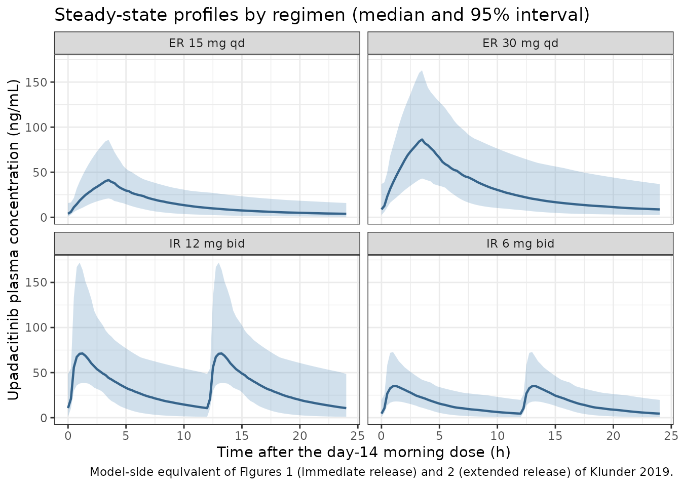
The two ER panels show the shape the mixed absorption model produces: a rounded peak near the end of the 3.29 h zero-order input, then a shallow decline sustained by the slow first-order arm - visibly flatter than the sharp twice-daily IR peaks, which is the property that motivated the ER tablet.
PKNCA validation
# Only `!is.na(Cc)` -- adding `time > 0` or `Cc > 0` would drop the row that
# anchors the interval and trigger PKNCA's "AUC range starting before the
# first measurement" warning on every subject.
sim_nca <- sim |>
  dplyr::filter(!is.na(Cc)) |>
  dplyr::select(id, time, Cc, regimen) |>
  dplyr::arrange(id, time)

conc_obj <- PKNCA::PKNCAconc(sim_nca, Cc ~ time | regimen + id)

# One dose row per administration. The ER arm carries two event records per
# administration (depot + central); PKNCA must see the administered amount
# once, so the central record is dropped here.
dose_df <- events |>
  dplyr::filter(evid == 1, cmt == "depot") |>
  dplyr::select(id, time, amt, regimen)

dose_obj <- PKNCA::PKNCAdose(dose_df, amt ~ time | regimen + id)

# Steady-state daily interval: the final 24 h, which is one dosing interval for
# the once-daily ER arms and two for the twice-daily IR arms. Using a common
# 24 h window makes the daily-AUC comparison direct.
intervals <- data.frame(
  start = t_last,
  end = t_last + 24,
  cmax = TRUE,
  cmin = TRUE,
  tmax = TRUE,
  auclast = TRUE
)

nca_res <- PKNCA::pk.nca(PKNCA::PKNCAdata(conc_obj, dose_obj, intervals = intervals))

nca_wide <- as.data.frame(nca_res) |>
  dplyr::filter(PPTESTCD %in% c("cmax", "cmin", "tmax", "auclast")) |>
  dplyr::select(regimen, id, PPTESTCD, PPORRES) |>
  tidyr::pivot_wider(names_from = PPTESTCD, values_from = PPORRES)
stopifnot(nrow(nca_wide) == 4L * n_arm)

nca_summary <- nca_wide |>
  dplyr::group_by(regimen) |>
  dplyr::summarise(
    cmax = median(cmax),
    cmin = median(cmin),
    tmax = median(tmax),
    auclast = median(auclast),
    .groups = "drop"
  )

nca_summary |>
  dplyr::rename(
    "Regimen" = regimen,
    "Cmax (ng/mL)" = cmax,
    "Cmin (ng/mL)" = cmin,
    "Tmax (h)" = tmax,
    "Daily AUC (ng*h/mL)" = auclast
  ) |>
  knitr::kable(
    digits = 2,
    caption = "Median steady-state non-compartmental parameters over the final 24 h (n = 100 per arm). The 24 h window spans TWO doses for the twice-daily IR arms, so their Tmax of about 13 h is the peak after the second (evening) dose of the day, not a delayed first peak; their Cmax is the larger of the two daily peaks and their 'daily AUC' covers both dosing intervals."
)| Regimen | Cmax (ng/mL) | Cmin (ng/mL) | Tmax (h) | Daily AUC (ng*h/mL) |
|---|---|---|---|---|
| ER 15 mg qd | 41.28 | 3.88 | 3.50 | 357.29 |
| ER 30 mg qd | 86.29 | 8.76 | 3.50 | 758.35 |
| IR 12 mg bid | 71.44 | 10.63 | 13.25 | 761.98 |
| IR 6 mg bid | 35.48 | 4.52 | 13.25 | 382.02 |
Comparison against the published bridging claim
Klunder 2019 reports no NCA table of its own, so the reference values
below are the ratios its Introduction asserts between the ER
and IR regimens, citing the dedicated phase I comparison. The model-side
ratio of daily AUC is a pure consequence of the relative bioavailability
and the daily dose: 0.762 x 15 / 12 = 0.9525 for the low
pair and 0.762 x 30 / 24 = 0.9525 for the high pair - both
within 5% of unity, which is what “equivalent daily AUC” means here.
ratio_of <- function(er_regimen, ir_regimen, col) {
  nca_summary[[col]][nca_summary$regimen == er_regimen] /
    nca_summary[[col]][nca_summary$regimen == ir_regimen]
}

bridging <- tibble::tribble(
  ~Comparison, ~Metric, ~`Simulated ratio`, ~`Closed-form / published expectation`,
  "ER 15 qd vs IR 6 bid", "Daily AUC", ratio_of("ER 15 mg qd", "IR 6 mg bid", "auclast"), 0.762 * 15 / 12,
  "ER 30 qd vs IR 12 bid", "Daily AUC", ratio_of("ER 30 mg qd", "IR 12 mg bid", "auclast"), 0.762 * 30 / 24,
  "ER 15 qd vs IR 6 bid", "Cmax", ratio_of("ER 15 mg qd", "IR 6 mg bid", "cmax"), NA_real_,
  "ER 30 qd vs IR 12 bid", "Cmax", ratio_of("ER 30 mg qd", "IR 12 mg bid", "cmax"), NA_real_,
  "ER 15 qd vs IR 6 bid", "Cmin", ratio_of("ER 15 mg qd", "IR 6 mg bid", "cmin"), NA_real_,
  "ER 30 qd vs IR 12 bid", "Cmin", ratio_of("ER 30 mg qd", "IR 12 mg bid", "cmin"), NA_real_
)
knitr::kable(bridging, digits = 3,
caption = "Extended-release versus immediate-release steady-state exposure ratios. Klunder 2019 Introduction: ER 15 and 30 mg qd give equivalent daily AUC and comparable Cmax and Cmin to IR 6 and 12 mg bid.")| Comparison | Metric | Simulated ratio | Closed-form / published expectation |
|---|---|---|---|
| ER 15 qd vs IR 6 bid | Daily AUC | 0.935 | 0.953 |
| ER 30 qd vs IR 12 bid | Daily AUC | 0.995 | 0.953 |
| ER 15 qd vs IR 6 bid | Cmax | 1.164 | NA |
| ER 30 qd vs IR 12 bid | Cmax | 1.208 | NA |
| ER 15 qd vs IR 6 bid | Cmin | 0.860 | NA |
| ER 30 qd vs IR 12 bid | Cmin | 0.824 | NA |
The table above compares medians of four independent 100-subject cohorts, so each ratio carries the sampling noise of two separate eta draws. The tight gate on daily AUC therefore uses the typical subject instead, where the comparison is paired by construction and the answer is exact arithmetic.
# Steady-state daily AUC for the typical RA subject at the reference
# covariates. With no random effects the four regimens differ only in dose,
# formulation and dosing frequency, so this isolates the bridging claim from
# cohort noise.
daily_auc_typical <- function(amt, tau, er) {
  cov <- list(WT = 74, CRCL = 108.70, DIS_RA = 1, STUDY_UPA_PHASE1 = 0)
  # The observed window is 24 h wide, so a twice-daily arm must receive BOTH of
  # its doses inside it; dosing only `until = t_last` would drop the evening
  # dose and understate the IR daily AUC by nearly half (it inflates the ratio
  # below from 0.95 to 1.65). This matches `dose_times` in `make_arm()`.
  last_dose <- t_last + (tau < 24) * tau
  ev <- rxode2::et(amt = amt, ii = tau, until = last_dose, cmt = "depot")
  if (er) {
    ev <- rxode2::et(ev, amt = amt, ii = tau, until = last_dose,
                     cmt = "central", rate = -2)
  }
  ev <- rxode2::et(ev, seq(t_last, t_last + 24, by = 0.02))
  d <- as.data.frame(ev)
  for (nm in names(cov)) d[[nm]] <- cov[[nm]]
  d$FORM_UPA_ER <- as.integer(er)
  s <- rxode2::rxSolve(mod_typ, d, returnType = "data.frame")
  o <- s[!is.na(s$Cc) & s$time >= t_last, ]
  sum(diff(o$time) * (head(o$Cc, -1) + tail(o$Cc, -1)) / 2)
}

typ_ratio <- c(
  `ER 15 qd / IR 6 bid` = daily_auc_typical(15, 24, TRUE) / daily_auc_typical(6, 12, FALSE),
  `ER 30 qd / IR 12 bid` = daily_auc_typical(30, 24, TRUE) / daily_auc_typical(12, 12, FALSE)
)
#> ℹ omega/sigma items treated as zero: 'etalcl_ph1', 'etalcl_ph23', 'etalvc_ph1', 'etalvc_ph23', 'etalka_er'
#> ℹ omega/sigma items treated as zero: 'etalcl_ph1', 'etalcl_ph23', 'etalvc_ph1', 'etalvc_ph23', 'etalka_er'
#> ℹ omega/sigma items treated as zero: 'etalcl_ph1', 'etalcl_ph23', 'etalvc_ph1', 'etalvc_ph23', 'etalka_er'
#> ℹ omega/sigma items treated as zero: 'etalcl_ph1', 'etalcl_ph23', 'etalvc_ph1', 'etalvc_ph23', 'etalka_er'
typ_ratio
#>  ER 15 qd / IR 6 bid ER 30 qd / IR 12 bid
#>            0.9525184            0.9525184
# Closed form: F_rel * (daily ER dose) / (daily IR dose) = 0.762 * 15/12 =
# 0.762 * 30/24 = 0.9525 exactly, for both pairs. This is deterministic, so
# the tolerance is numerical only -- both ratios realise 0.952518, i.e. within
# 2e-5 of the closed form, so 1e-3 leaves ~50x headroom for solver and grid
# differences across platforms while still going red on a mis-transcribed
# relative bioavailability (0.762 -> 1.0 would give 1.25), a broken dose split,
# or a dropped dose (see the `last_dose` comment above: that gives 1.65).
stopifnot(all(abs(typ_ratio - 0.9525) < 0.001))
cmax_ratios <- c(
  ratio_of("ER 15 mg qd", "IR 6 mg bid", "cmax"),
  ratio_of("ER 30 mg qd", "IR 12 mg bid", "cmax")
)
cmin_ratios <- c(
  ratio_of("ER 15 mg qd", "IR 6 mg bid", "cmin"),
  ratio_of("ER 30 mg qd", "IR 12 mg bid", "cmin")
)
auc_ratios <- c(
  ratio_of("ER 15 mg qd", "IR 6 mg bid", "auclast"),
  ratio_of("ER 30 mg qd", "IR 12 mg bid", "auclast")
)

# Cohort-level bands. These compare medians of independent cohorts, so they are
# deliberately wide -- they exist to catch a structurally broken absorption
# model, not to re-measure the closed form above. Dropping the zero-order arm
# entirely takes the Cmax ratio below 0.3 and the daily-AUC ratio to about
# 0.24, so all three bands can still go red.
stopifnot(all(auc_ratios > 0.8), all(auc_ratios < 1.15))
stopifnot(all(cmax_ratios > 0.6), all(cmax_ratios < 1.6))
stopifnot(all(cmin_ratios > 0.5), all(cmin_ratios < 2.0))
The typical-subject daily-AUC ratio lands on the closed-form 0.9525 for both dose pairs, and the cohort peak and trough ratios sit near unity, reproducing the bridging claim.
Steady-state dose proportionality
Klunder 2019 Discussion states upadacitinib bioavailability “was dose-proportional over the evaluated ER dose range of 7.5-30 mg”, and the model is linear, so doubling the dose must double the exposure within each formulation.
prop_auc <- c(
  IR = nca_summary$auclast[nca_summary$regimen == "IR 12 mg bid"] /
    nca_summary$auclast[nca_summary$regimen == "IR 6 mg bid"],
  ER = nca_summary$auclast[nca_summary$regimen == "ER 30 mg qd"] /
    nca_summary$auclast[nca_summary$regimen == "ER 15 mg qd"]
)
prop_auc
#>       IR       ER
#> 1.994617 2.122525
# Each arm is an independent draw of 100 subjects, so the ratio of medians is
# 2 plus cohort noise rather than exactly 2.
stopifnot(all(abs(prop_auc - 2) < 0.25))
Assumptions and deviations
-
Centering (reference) covariate values are not printed by
Klunder 2019. The paper states that continuous covariates
entered “centered on the median covariate value” but reports only means
in Table 2 (76.4 kg, 113.7 mL/min) and carries no centering footnote in
Table 3.
ref_wt = 74 kgandref_crcl = 108.70 mL/minare taken from the NONMEM control stream in Appendix S1 of Bhatnagar 2024 (Clin Transl Sci 17:e13733), aMAXEVAL = 0evaluation of this same model, and are corroborated by that paper’s Table S3 footnote b. These are therefore not paper-derived values in the strict sense - they come from a successor publication’s supplement, not from Klunder 2019 itself. They cancel out of every exposure ratio, so no check in this vignette depends on them; they set only the absolute typical value for an off-reference subject. -
DIS_RAversusDIS_HEALTHY. This model uses the canonicalDIS_RA(1 = RA patient) because the source column is literallyRAcoded 1 = RA and the contrast maps onto the canonical orientation with no transformation. The two sibling upadacitinib models use the complementaryDIS_HEALTHYcolumn -Klunder_2017_upadacitinibbecause it gates paired healthy/RA structural means rather than applying a single multiplier, andBhatnagar_2024_upadacitinibbecause its patient cohort is axial spondyloarthritis rather than RA. Set both consistently if you pool simulations across the three models. -
The phase I / phase II-III split is a variance stratum, not
a disease stratum.
STUDY_UPA_PHASE1selects only the ISV magnitudes on CL/F and Vc/F and the proportional residual-error magnitude; it changes no typical value. It is not interchangeable withDIS_RA: 14 of the 188 phase I subjects had RA, and the RA clearance effect is carried separately. A model needs both columns. -
Retained convention-lint warning on
e_ra_cl.checkModelConventions()flagse_ra_clas possibly reversed (e_<param>_<cov>instead of the canonicale_<cov>_<param>). It is a false positive from the heuristic: the covariate token israand the parameter token iscl, which is canonical order. The name is kept because it is the established spelling for this exact covariate/parameter pair in the register’s otherDIS_RAmodels –Li_2018_PF04236921.Rand bothWojciechowski_2023_ritlecitinib_*.Rfiles all usee_ra_clfor the RA-on-clearance effect. The only other lint output is an informational note thatunits$dosing(mg) andunits$concentration(ng/mL) differ in magnitude; the model applies the explicit1000 *factor inCc. - No CL/F-Vc/F correlation is reported for this model, so the etas are simulated independently. (The successor axSpA analysis does report a covariance of -0.160 in its control stream, but that belongs to its own re-estimated variance structure, not to this one.)
-
ISV on the immediate-release Ka could not be
estimated. Klunder 2019 Results: “The estimation of ISV
variability on the Ka of the IR formulation was not numerically feasible
with the current dataset.” The model therefore carries a random effect
on the ER
Kaonly, exactly as published; the IR absorption rate is a typical value for every subject. - The virtual cohort’s covariate distributions are approximations. Body weight and creatinine clearance are drawn as truncated normals matching the Table 2 means, SDs and observed ranges. The paper reports no correlation between them and no full joint distribution, so they are drawn independently; in reality they are positively correlated through the Cockcroft-Gault weight term, which would slightly narrow the simulated exposure spread.
-
No published NCA table exists in this paper to
compare against directly. The validation therefore uses (a) exact
closed-form dose-recovery identities,
- the abstract’s own ER clearance and steady-state volume, (c) an inversion of the Figure 4 forest-plot ratios back onto the paper’s covariate bands, and
- the ER-versus-IR bridging claim stated in the Introduction. Sections needing per-group observed Cmax / AUC values are omitted because the source does not report them.
- Outlier and BLQ handling is not reproduced. The published fit set BLQ values to LLOQ/2 (M5), censored repeat post-dose BLQ records, dropped observations beyond 168 h after the last dose, and excluded 1.7% of records by an ANOVA-based outlier rule (Klunder 2019 supplementary Methods). None of that affects a forward simulation from the final parameter estimates.