Oxycodone, noroxycodone and noroxymorphone (Agema 2021)
Source:vignettes/articles/Agema_2021_oxycodone.Rmd
Agema_2021_oxycodone.RmdModel and source
- Citation: Agema BC, Oosten AW, Sassen SDT, Rietdijk WJR, van der Rijt CCD, Koch BCP, Mathijssen RHJ, Koolen SLW. Population Pharmacokinetics of Oxycodone and Metabolites in Patients with Cancer-Related Pain. Cancers (Basel). 2021;13(11):2768. doi:10.3390/cancers13112768
- Description: Joint one-compartment population PK model for oral oxycodone and its sequential N-demethylated metabolites noroxycodone and noroxymorphone in hospitalised adults with cancer-related pain (Agema 2021). Immediate- release (IR) and extended-release (ER) tablets are dosed into two separate first-order absorption depots (depot = IR, depot2 = ER); oxycodone is eliminated by a fixed first-order route and converted by a first-order rate constant to noroxycodone, which is eliminated and further converted to noroxymorphone. The model is parameterised in micro-rate constants and apparent volumes, with IIV on the two formation/elimination constants of noroxycodone and on noroxymorphone elimination, and no covariates. DOSES ARE IN MMOL OF OXYCODONE and all three concentrations are in nmol/L, as in the authors’ NONMEM dataset: 10 mg oxycodone (free base, MW 315.36 g/mol) is 0.03171 mmol.
- Article: https://doi.org/10.3390/cancers13112768 (open access)
- Supplement: https://www.mdpi.com/article/10.3390/cancers13112768/s1 (Document S1 covariate equations; Document S2 control stream of the final model)
Agema et al. fitted one NONMEM model jointly to plasma oxycodone and
its two N-demethylated metabolites, noroxycodone and noroxymorphone, in
hospitalised patients with cancer-related pain. Immediate-release (IR)
and extended-release (ER) tablets enter separate first-order absorption
depots. Oxycodone is removed by a fixed first-order route
(K30) and converted to noroxycodone (K34).
Noroxycodone is eliminated (K40) and converted to
noroxymorphone (K45), which is then eliminated
(K50). Oxymorphone was measured but not modelled, because
more than half of its samples were below the limit of quantification. No
covariate was retained.
Units. The model is in the authors’ dataset units.
Doses are in mmol of oxycodone and all three
concentrations are in nmol/L: Document S2 scales with
S3 = V3/1000000 (“scaling from nmol/L (observations) to
mmol (dosages)”). A 10 mg tablet is entered as
10 / 315.36 = 0.03171 mmol (see Assumptions and
deviations for the molecular weight).
Population
The analysis included 28 hospitalised adults (one enrolled twice) with moderate to severe nociceptive cancer-related pain, treated at the Erasmus MC Cancer Institute, Rotterdam. Their median age was 62.5 years (range 39-81) and median weight 80.0 kg (46-135); 43% were female. Primary tumours were urogenital (32%), breast (18%), GIST or soft-tissue sarcoma (14%), melanoma (11%) and other (25%). Median eGFR was 86.0 mL/min (37 to >90) and median albumin 42.5 g/L. No patient had Child-Pugh B or C liver dysfunction. There were 12 CYP2D6 extensive and 10 intermediate metabolizers (6 missing), 6 CYP3A4*22 heterozygotes, and 17 UGT2B7*2 heterozygotes and 5 homozygous variants (Table 1). ER tablets were dosed at 5-100 mg twice daily (08:00 and 20:00) and IR tablets at 5-30 mg as needed. In all, 302 samples gave 1207 measurements, of which 29.2% were below the limit of quantification and were handled with the M3 method.
The same information is available programmatically via
readModelDb("Agema_2021_oxycodone")()$population.
Source trace
Each ini() value also carries its source as an in-file
comment in
inst/modeldb/specificDrugs/Agema_2021_oxycodone.R.
| Equation / parameter | Value | Source location |
|---|---|---|
lka_ir (Ka,IR, NONMEM K13) |
log(3.61) 1/h | Table 2 |
lka_er (Ka,ER, NONMEM K23) |
log(0.329) 1/h | Table 2 (row label printed as ‘Ka, ER 23’) |
lvc (V3/F) |
log(619) L | Table 2 |
lkel (K30) |
fixed(log(0.01224)) 1/h | Table 2 prints 0.012 FIX; Document S2 $THETA(3) =
0.01224 FIX |
lkmet_noroxycod (K34) |
log(0.086) 1/h | Table 2 |
lvc_noroxycod (V4/F) |
fixed(log(16.3)) L | Table 2; Document S2 $THETA(7)
|
lkel_noroxycod (K40) |
log(3.28) 1/h | Table 2 |
lkmet_noroxymor (K45) |
log(1.36) 1/h | Table 2 |
lvc_noroxymor (V5/F) |
fixed(log(64.1)) L | Table 2; Document S2 $THETA(12)
|
lkel_noroxymor (K50) |
log(1.97) 1/h | Table 2 |
etalkmet_noroxycod |
0.1200 = log(1 + 0.357^2) | Table 2, IIV K34 35.7 CV% |
etalkel_noroxycod |
0.6801 = log(1 + 0.987^2) | Table 2, IIV K40 98.7 CV% |
etalkel_noroxymor |
0.5113 = log(1 + 0.817^2) | Table 2, IIV K50 81.7 CV% |
propSd |
0.397 | Table 2 (oxycodone additive 0 FIX) |
propSd_noroxycod, addSd_noroxycod
|
0.167, 3.34 nM | Table 2 |
propSd_noroxymor, addSd_noroxymor
|
0.156, 1.09 nM | Table 2 |
combined1() error form |
SD = prop * IPRED + add | Document S2 $ERROR:
W = IPRED*THETA(prop) + THETA(add),
$SIGMA 1 FIX
|
ODEs for depot, depot2,
central, central_noroxycod,
central_noroxymor
|
n/a | Document S2 $DES; Figure 2 |
Cc = 1e6 * central / vc (and metabolites) |
n/a | Document S2 S3 = V3/1000000 (mmol dose, nmol/L
observation) |
Closed-form checks
With first-order kinetics throughout, the steady-state exposure
ratios follow directly from the parameters. Over a dosing interval,
AUC_noroxycod / AUC_oxy = K34 * V3 / ((K40 + K45) * V4) and
AUC_noroxymor / AUC_oxy = (AUC_noroxycod / AUC_oxy) * K45 * V4 / (K50 * V5).
Oxycodone’s apparent clearance is (K30 + K34) * V3. The
Discussion states that “the AUC of nor-oxymorphone was eight times lower
than the AUC of oxycodone” and “the AUC of nor-oxycodone was two thirds
that of oxycodone”. Both statements are checks on the whole parameter
chain that do not depend on the dose’s molecular weight.
mod <- readModelDb("Agema_2021_oxycodone")
p <- rxode2::rxode(mod)$theta
#> ℹ parameter labels from comments will be replaced by 'label()'
k30 <- exp(p[["lkel"]])
k34 <- exp(p[["lkmet_noroxycod"]])
k40 <- exp(p[["lkel_noroxycod"]])
k45 <- exp(p[["lkmet_noroxymor"]])
k50 <- exp(p[["lkel_noroxymor"]])
v3 <- exp(p[["lvc"]])
v4 <- exp(p[["lvc_noroxycod"]])
v5 <- exp(p[["lvc_noroxymor"]])

cl_oxy <- (k30 + k34) * v3
ratio_noroxycod <- k34 * v3 / ((k40 + k45) * v4)
ratio_noroxymor <- ratio_noroxycod * k45 * v4 / (k50 * v5)
thalf_oxy <- log(2) / (k30 + k34)

closed <- tibble::tibble(
  quantity = c(
    "Oxycodone CL/F (L/h)",
    "Oxycodone half-life (h)",
    "AUC noroxycodone / AUC oxycodone",
    "AUC oxycodone / AUC noroxymorphone"
  ),
  model = c(cl_oxy, thalf_oxy, ratio_noroxycod, 1 / ratio_noroxymor),
  paper = c(NA, NA, 2 / 3, 8)
)
knitr::kable(closed, digits = 3, caption = "Closed-form typical values against the Discussion's statements.")| quantity | model | paper |
|---|---|---|
| Oxycodone CL/F (L/h) | 60.811 | NA |
| Oxycodone half-life (h) | 7.056 | NA |
| AUC noroxycodone / AUC oxycodone | 0.704 | 0.667 |
| AUC oxycodone / AUC noroxymorphone | 8.093 | 8.000 |
Virtual cohort and simulation
Two regimens are simulated: a single 5 mg IR tablet, and ER 10 mg every 12 h (the median ER dose at inclusion, Table 1) for 7 days, which reaches steady state for all three analytes (oxycodone half-life about 7 h). The model has no covariates, so the virtual patients differ only in their random effects. Each arm has 200 patients.
mw_oxycodone <- 315.36 # g/mol, free base
mg_to_mmol <- function(mg) mg / mw_oxycodone

tau <- 12
n_er_doses <- 14
ss_start <- tau * (n_er_doses - 1)

obs_ir <- sort(unique(c(seq(0, 2, by = 0.05), seq(2, 12, by = 0.25), seq(12, 72, by = 1))))
obs_er <- sort(unique(c(seq(0, ss_start, by = 2), ss_start + seq(0, tau, by = 0.05))))

make_arm <- function(n, arm, id_offset) {
  ids <- id_offset + seq_len(n)
  if (arm == "IR 5 mg single dose") {
    dose <- tibble::tibble(id = ids, time = 0, amt = mg_to_mmol(5), cmt = "depot", evid = 1L)
    obs_times <- obs_ir
  } else {
    dose <- tidyr::expand_grid(id = ids, time = tau * (seq_len(n_er_doses) - 1)) |>
      dplyr::mutate(amt = mg_to_mmol(10), cmt = "depot2", evid = 1L)
    obs_times <- obs_er
  }
  # Observation rows sit on the oxycodone ODE state with dvid = 1 (the first
  # endpoint, Cc). The model has three endpoints, so an observation row with
  # no dvid cannot be mapped; the metabolite concentrations are still returned
  # as columns on every row.
  obs <- tidyr::expand_grid(id = ids, time = obs_times) |>
    dplyr::mutate(amt = 0, cmt = "central", evid = 0L, dvid = 1L)
  dplyr::bind_rows(dose, obs) |>
    dplyr::mutate(treatment = arm) |>
    dplyr::arrange(id, time, dplyr::desc(evid))
}

arms <- c("IR 5 mg single dose", "ER 10 mg q12h")
events_typ <- dplyr::bind_rows(
  make_arm(1, arms[1], id_offset = 0L),
  make_arm(1, arms[2], id_offset = 1L)
)
events <- dplyr::bind_rows(
  make_arm(200, arms[1], id_offset = 0L),
  make_arm(200, arms[2], id_offset = 200L)
)
stopifnot(!anyDuplicated(unique(events[, c("id", "time", "evid")])))
rxode2::rxSetSeed(20210602)
sim_typ <- rxode2::rxSolve(
  rxode2::zeroRe(mod),
  events = events_typ, keep = "treatment", useLinCmt = FALSE
) |>
  as.data.frame()
#> ℹ parameter labels from comments will be replaced by 'label()'
#> ℹ omega/sigma items treated as zero: 'etalkmet_noroxycod', 'etalkel_noroxycod', 'etalkel_noroxymor'
#> Warning: multi-subject simulation without without 'omega'
sim <- rxode2::rxSolve(mod, events = events, keep = "treatment", useLinCmt = FALSE) |>
  as.data.frame()
#> ℹ parameter labels from comments will be replaced by 'label()'

to_long <- function(d) {
  d |>
    dplyr::select(id, time, treatment, Cc, Cc_noroxycod, Cc_noroxymor) |>
    tidyr::pivot_longer(c(Cc, Cc_noroxycod, Cc_noroxymor), names_to = "analyte", values_to = "conc") |>
    dplyr::mutate(analyte = dplyr::recode(
      analyte,
      Cc = "Oxycodone", Cc_noroxycod = "Noroxycodone", Cc_noroxymor = "Noroxymorphone"
    ))
}
long_typ <- to_long(sim_typ)
long <- to_long(sim)
Replicate published figures
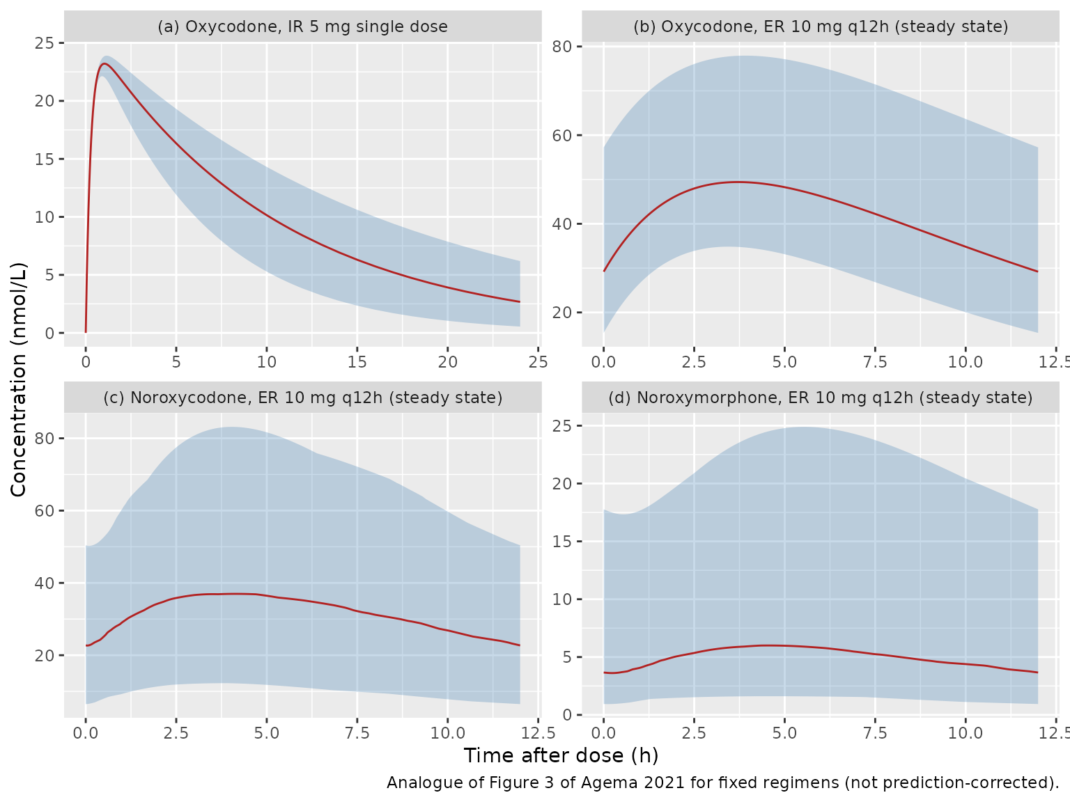
Figure 3 of Agema 2021 shows prediction-corrected VPCs pooled over each patient’s own IR / ER doses (5-100 mg) and sampling times, so it cannot be reproduced exactly without the observed data. The panels below show the same four views for the two fixed regimens above: the median and the 5th-95th percentile band against time after dose. They are for checking scale and shape. The paper’s pooled medians are about 50-120 nmol/L for oxycodone, a noroxycodone peak of about 70 nmol/L near 2-3 h after dose, and a noroxymorphone peak of about 20 nmol/L near 4 h.
vpc <- long |>
  dplyr::filter(treatment == arms[1] | time >= ss_start) |>
  dplyr::mutate(
    tad = ifelse(treatment == arms[1], time, time - ss_start),
    panel = dplyr::case_when(
      analyte == "Oxycodone" & treatment == arms[1] ~ "(a) Oxycodone, IR 5 mg single dose",
      analyte == "Oxycodone" ~ "(b) Oxycodone, ER 10 mg q12h (steady state)",
      analyte == "Noroxycodone" & treatment == arms[2] ~ "(c) Noroxycodone, ER 10 mg q12h (steady state)",
      analyte == "Noroxymorphone" & treatment == arms[2] ~ "(d) Noroxymorphone, ER 10 mg q12h (steady state)",
      TRUE ~ NA_character_
    )
  ) |>
  dplyr::filter(!is.na(panel), tad <= 24) |>
  dplyr::group_by(panel, tad) |>
  dplyr::summarise(
    Q05 = quantile(conc, 0.05),
    Q50 = quantile(conc, 0.50),
    Q95 = quantile(conc, 0.95),
    .groups = "drop"
  )

ggplot(vpc, aes(tad, Q50)) +
  geom_ribbon(aes(ymin = Q05, ymax = Q95), fill = "steelblue", alpha = 0.3) +
  geom_line(colour = "firebrick") +
  facet_wrap(~panel, scales = "free") +
  labs(
    x = "Time after dose (h)", y = "Concentration (nmol/L)",
    caption = "Analogue of Figure 3 of Agema 2021 for fixed regimens (not prediction-corrected)."
  )
PKNCA validation
PKNCA is run on the typical-value (zeroRe()) profiles,
once per analyte, for the IR single dose (terminal half-life) and for
the last ER interval at steady state (AUCtau).
run_nca <- function(d, dose_df, intervals) {
  conc <- d |>
    dplyr::filter(!is.na(conc)) |>
    dplyr::select(id, time, conc, treatment)
  conc <- dplyr::bind_rows(
    conc,
    conc |> dplyr::distinct(id, treatment) |> dplyr::mutate(time = 0, conc = 0)
  ) |>
    dplyr::distinct(id, treatment, time, .keep_all = TRUE) |>
    dplyr::arrange(id, treatment, time)
  conc_obj <- PKNCA::PKNCAconc(conc, conc ~ time | treatment + id)
  dose_obj <- PKNCA::PKNCAdose(dose_df, amt ~ time | treatment + id)
  res <- PKNCA::pk.nca(PKNCA::PKNCAdata(conc_obj, dose_obj, intervals = intervals))
  as.data.frame(res$result)
}

dose_typ <- events_typ |>
  dplyr::filter(evid == 1) |>
  dplyr::select(id, time, amt, treatment)

nca_typ <- lapply(c("Oxycodone", "Noroxycodone", "Noroxymorphone"), function(a) {
  d <- dplyr::filter(long_typ, analyte == a)
  ir <- run_nca(
    dplyr::filter(d, treatment == arms[1]),
    dplyr::filter(dose_typ, treatment == arms[1]),
    data.frame(start = 0, end = 72, cmax = TRUE, tmax = TRUE, half.life = TRUE)
  )
  er <- run_nca(
    dplyr::filter(d, treatment == arms[2]),
    dplyr::filter(dose_typ, treatment == arms[2]),
    data.frame(start = ss_start, end = ss_start + tau, auclast = TRUE, cmax = TRUE, tmax = TRUE)
  )
  dplyr::bind_rows(ir, er) |> dplyr::mutate(analyte = a)
}) |>
  dplyr::bind_rows()

nca_wide <- nca_typ |>
  dplyr::filter(PPTESTCD %in% c("cmax", "tmax", "half.life", "auclast")) |>
  dplyr::select(analyte, treatment, PPTESTCD, PPORRES) |>
  tidyr::pivot_wider(names_from = PPTESTCD, values_from = PPORRES)

nca_wide |>
  dplyr::rename(
    "Analyte" = analyte,
    "Regimen" = treatment,
    "Cmax (nmol/L)" = cmax,
    "Tmax (h)" = tmax,
    "t1/2 (h)" = half.life,
    "AUCtau (nmol*h/L)" = auclast
  ) |>
knitr::kable(digits = 2, caption = "Typical-value NCA (PKNCA).")| Analyte | Regimen | Cmax (nmol/L) | Tmax (h) | t1/2 (h) | AUCtau (nmol*h/L) |
|---|---|---|---|---|---|
| Oxycodone | IR 5 mg single dose | 23.15 | 1.05 | 7.06 | NA |
| Oxycodone | ER 10 mg q12h | 51.29 | 3.75 | NA | 521.45 |
| Noroxycodone | IR 5 mg single dose | 16.07 | 1.35 | 7.06 | NA |
| Noroxycodone | ER 10 mg q12h | 36.07 | 3.95 | NA | 367.03 |
| Noroxymorphone | IR 5 mg single dose | 2.66 | 2.25 | 7.06 | NA |
| Noroxymorphone | ER 10 mg q12h | 6.30 | 4.50 | NA | 64.43 |
The paper reports no NCA table, so there is no side-by-side NCA comparison. The checks below compare the PKNCA results with the model’s closed forms (mass balance and exposure ratios) and with the two exposure ratios stated in the Discussion.
get_val <- function(a, trt, code) {
  nca_typ$PPORRES[nca_typ$analyte == a & nca_typ$treatment == trt & nca_typ$PPTESTCD == code]
}
auc_oxy <- get_val("Oxycodone", arms[2], "auclast")
auc_noroxycod <- get_val("Noroxycodone", arms[2], "auclast")
auc_noroxymor <- get_val("Noroxymorphone", arms[2], "auclast")

gates <- tibble::tibble(
  check = c(
    "CL/F * AUCtau(oxycodone) / dose (mass balance)",
    "AUCtau ratio noroxycodone / oxycodone vs closed form",
    "AUCtau ratio noroxymorphone / oxycodone vs closed form",
    "Oxycodone t1/2 vs log(2) / (K30 + K34)",
    "Noroxycodone terminal t1/2 vs oxycodone (formation-rate limited)",
    "Noroxymorphone terminal t1/2 vs oxycodone (formation-rate limited)"
  ),
  value = c(
    cl_oxy * auc_oxy / 1e6 / mg_to_mmol(10),
    (auc_noroxycod / auc_oxy) / ratio_noroxycod,
    (auc_noroxymor / auc_oxy) / ratio_noroxymor,
    get_val("Oxycodone", arms[1], "half.life") / thalf_oxy,
    get_val("Noroxycodone", arms[1], "half.life") / thalf_oxy,
    get_val("Noroxymorphone", arms[1], "half.life") / thalf_oxy
  )
)
knitr::kable(gates, digits = 4, caption = "Ratios that should equal 1.")| check | value |
|---|---|
| CL/F * AUCtau(oxycodone) / dose (mass balance) | 1.0000 |
| AUCtau ratio noroxycodone / oxycodone vs closed form | 1.0000 |
| AUCtau ratio noroxymorphone / oxycodone vs closed form | 1.0000 |
| Oxycodone t1/2 vs log(2) / (K30 + K34) | 1.0005 |
| Noroxycodone terminal t1/2 vs oxycodone (formation-rate limited) | 1.0007 |
| Noroxymorphone terminal t1/2 vs oxycodone (formation-rate limited) | 1.0005 |
# These compare a typical-value solve with its own closed form, so the only
# difference is numerical (grid and trapezoid) error; tight bounds are correct.
stopifnot(all(abs(gates$value - 1) < 0.02))
The metabolite half-lives equal the parent’s because both metabolites
are eliminated much faster (K40 + K45 = 4.64 1/h,
K50 = 1.97 1/h) than oxycodone
(K30 + K34 = 0.098 1/h). Their concentrations are
formation-rate limited and follow the parent’s terminal decline.
Between-patient spread of metabolite exposure
In the stochastic cohort, each patient’s steady-state noroxycodone /
oxycodone exposure ratio is
K34_i * V3 / ((K40_i + K45) * V4). Its median should lie
close to the typical value, and its spread shows the variability carried
by the IIV on K34 and K40.
auc_ind <- long |>
  dplyr::filter(treatment == arms[2], time >= ss_start) |>
  dplyr::group_by(id, analyte) |>
  dplyr::summarise(
    auc = sum(diff(time) * (head(conc, -1) + tail(conc, -1)) / 2),
    .groups = "drop"
  ) |>
  tidyr::pivot_wider(names_from = analyte, values_from = auc) |>
  dplyr::mutate(
    r_noroxycod = Noroxycodone / Oxycodone,
    r_noroxymor = Noroxymorphone / Oxycodone
  )

ratio_summary <- tibble::tibble(
  ratio = c("noroxycodone / oxycodone", "noroxymorphone / oxycodone"),
  typical = c(ratio_noroxycod, ratio_noroxymor),
  median = c(median(auc_ind$r_noroxycod), median(auc_ind$r_noroxymor)),
  p05 = c(quantile(auc_ind$r_noroxycod, 0.05), quantile(auc_ind$r_noroxymor, 0.05)),
  p95 = c(quantile(auc_ind$r_noroxycod, 0.95), quantile(auc_ind$r_noroxymor, 0.95))
)
knitr::kable(ratio_summary, digits = 3, caption = "Steady-state AUCtau ratios across 200 simulated patients (ER 10 mg q12h).")| ratio | typical | median | p05 | p95 |
|---|---|---|---|---|
| noroxycodone / oxycodone | 0.704 | 0.697 | 0.202 | 1.989 |
| noroxymorphone / oxycodone | 0.124 | 0.121 | 0.030 | 0.547 |
# Centre-only gate (robust to which patients land in the tails). With
# lognormal K40 (omega^2 0.68) the median ratio sits a little below the
# typical-value ratio because 1 / (K40 + K45) is a concave transform; 25% is
# well outside that shift but far inside a transcription error in K34, K40 or V4.
stopifnot(abs(median(auc_ind$r_noroxycod) / ratio_noroxycod - 1) < 0.25)
Assumptions and deviations
- Dose molecular weight. The dataset carried doses in mmol of oxycodone (Document S2), but the paper does not say which molecular weight converted the tablet strength in mg to mmol. The stream’s LLOQ constants use free-base molecular weights for the concentrations (0.200 ng/mL / 315.36 g/mol = 0.6342 nmol/L). This vignette therefore converts doses with the oxycodone free-base weight of 315.36 g/mol. If the authors instead converted the labelled oxycodone hydrochloride strength with the salt weight (351.83 g/mol), a labelled dose corresponds to 10.4% fewer mmol, and simulated concentrations for a given labelled mg dose would be 10.4% lower. The model itself takes mmol and does not depend on this choice. The exposure ratios in the closed-form checks do not depend on it either.
-
IIV covariances omitted. Document S2 estimates a
full
$OMEGA BLOCK(3)on K34, K40 and K50. The paper prints only the three CV% values (Table 2), and the stream’s block holds initial estimates, so the final covariances are not available. The model encodes a diagonal omega matrix. -
CV% to variance. Table 2’s IIV CV% values are
converted with
omega^2 = log(1 + CV^2). The stream’s initial$OMEGAvalues (0.134, 0.277 and 0.03) are too far from the published finals to distinguish this reading fromomega^2 = CV^2, which would give 0.127, 0.974 and 0.667. The two readings differ materially only for K40 and K50. - K30 precision. Table 2 prints the fixed K30 as 0.012 1/h. The control stream fixes it at 0.01224 1/h, the value the final run used, and that value is encoded here.
-
Final estimates from Table 2. The stream’s
$THETArecords are initial estimates (for example V3 566 L vs the final 619 L). Every estimated parameter is taken from Table 2. -
Initial concentrations at inclusion. Two patients
had detectable oxycodone at inclusion. The authors set their compartment
amounts from the first observed concentrations (the
A_0block in Document S2). That is specific to the estimation dataset and is not part of the packaged model. Set initial conditions oncentral,central_noroxycodandcentral_noroxymor(in mmol) to reproduce it. - BLQ handling. The M3 likelihood for data below the limit of quantification is an estimation device and is not encoded. The stream’s LLOQs are 0.6342, 3.318511 and 3.480561 nmol/L for oxycodone, noroxycodone and noroxymorphone.
- Oxycodone additive error. It was fixed to 0 by the authors and is omitted, which leaves a proportional-only error for oxycodone.
- Excluded data. The authors discarded all ten noroxycodone samples from a patient who started dexamethasone mid-study (Results 3.1). The model describes noroxycodone without CYP3A4 induction.
- Errata. No correction notice was found for this article (Europe PMC search, 2026-09-28).