Propofol plasma and brain concentrations (Kawata 2024)
Source:vignettes/articles/Kawata_2024_propofol.Rmd
Kawata_2024_propofol.RmdModel and source
Kawata et al. (2024) measured propofol in arterial plasma and in brain tissue (lobectomy or uncapping margins) from patients undergoing awake craniotomy, and built two population PK models that predict both. Each model adds a brain compartment whose input carries a brain/plasma partition coefficient Kp, so that the predicted brain concentration can exceed the plasma concentration, which a classical effect compartment cannot do:
The paper’s two final models are packaged separately:
-
Kawata_2024_propofol_marsh– the extended Marsh model: the Marsh three-compartment micro-constants and weight-proportional central volume held fixed, with k1e, Kp and their variability estimated (Table 1). -
Kawata_2024_propofol_2cmt– the new model: a two-compartment PK model estimated from the paper’s own data, with the same brain compartment (Table 2).
mod_marsh <- readModelDb("Kawata_2024_propofol_marsh")
mod_2cmt <- readModelDb("Kawata_2024_propofol_2cmt")
ui_marsh <- rxode2::rxode(mod_marsh)
#> ℹ parameter labels from comments will be replaced by 'label()'
ui_2cmt <- rxode2::rxode(mod_2cmt)
#> ℹ parameter labels from comments will be replaced by 'label()'- Citation: Kawata M, Yonezawa A, Mineharu Y, Itohara K, Mizota T, Matsui Y, Kikuchi T, Yamao Y, Hattori EY, Hamada M, Hira D, Furukawa K, Miyamoto S, Terada T, Matsubara K, Arakawa Y. Development of extended pharmacokinetic models for propofol based on measured blood and brain concentrations. Sci Rep. 2024;14:6326. doi:10.1038/s41598-024-56863-z. PMCID: PMC10943190. Plasma PK fixed to the Marsh model (Marsh B, White M, Morton N, Kenny GN. Br J Anaesth. 1991;67:41-48. doi:10.1093/bja/67.1.41).
- Description (extended Marsh): Extended Marsh model for propofol plasma and brain concentrations in Japanese adults and adolescents undergoing awake craniotomy (Kawata 2024; N = 29 model-building patients). Three-compartment intravenous PK with the Marsh micro-constants and weight-proportional central volume fixed, plus a brain compartment whose input carries a brain/plasma partition coefficient Kp: dCbrain/dt = k1e * (Kp * Cc - Cbrain). k1e and Kp were estimated; IIV on k10, k13 and Kp; proportional error on plasma and additive error on brain concentrations; no covariates retained beyond the Marsh weight scaling.
- Description (new model): New two-compartment model for propofol plasma and brain concentrations in Japanese adults and adolescents undergoing awake craniotomy (Kawata 2024; N = 29 model-building patients). Two-compartment intravenous PK estimated from the paper’s own data, plus a brain compartment whose input carries a brain/plasma partition coefficient Kp: dCbrain/dt = k1e * (Kp * Cc - Cbrain). IIV on CL and Kp; proportional error on plasma and additive error on brain concentrations; no covariates retained.
- Article: https://doi.org/10.1038/s41598-024-56863-z (open access; the supplement contains both NONMEM control streams and the observed concentrations of all 57 patients)
Population
Ninety patients with brain tumours or other brain lesions underwent awake craniotomy at Kyoto University Hospital between May 2019 and June 2022; 57 had enough plasma and brain material for analysis. They were assigned in order of enrolment to a model-building group (the first 29 patients; 105 plasma and 80 brain concentrations) and a validation group (28 patients). In the model-building group (Supplementary Table S1) 16 were male and 13 female, the median age was 49 years (range 13-76), median weight 62.5 kg (44.0-92.8), median height 1.66 m and median BMI 21.7 kg/m^2; 26 of 29 had glioma. Samples were taken immediately before and 5, 15, 25 and 75 min after propofol was stopped to wake the patient.
str(ui_marsh$population)
#> List of 13
#>  $ species       : chr "human"
#>  $ n_subjects    : num 29
#>  $ n_studies     : num 1
#>  $ age_range     : chr "13-76 years"
#>  $ age_median    : chr "49 years"
#>  $ weight_range  : chr "44.0-92.8 kg"
#>  $ weight_median : chr "62.5 kg"
#>  $ sex_female_pct: num 44.8
#>  $ race_ethnicity: Named num 100
#>   ..- attr(*, "names")= chr "Asian"
#>  $ disease_state : chr "Brain tumour (glioma, 26/29) or other brain lesion (epilepsy, cavernous hemangioma, tuberculoma) undergoing awa"| __truncated__
#>  $ dose_range    : chr "Intravenous propofol infusion (target-controlled) until awakening; plasma (radial artery) and brain (lobectomy "| __truncated__
#>  $ regions       : chr "Japan (Kyoto University Hospital)"
#>  $ notes         : chr "Model-building group = first 29 of 57 consecutively enrolled patients (May 2019 - June 2022); the remaining 28 "| __truncated__
Source trace
Every ini() value carries an in-file comment pointing to
its source; the table collects them.
| Model | Equation / parameter | Value | Source location |
|---|---|---|---|
| both | d/dt(brain) <- ke0 * kp_brain * Cc - ke0 * brain |
n/a | Methods, brain-compartment equation; ke0’ = k1e; Supplementary codes
1 and 2 $DES
|
| both | brain observed as a concentration, density 1 g/mL | n/a | Methods; NONMEM brain state observed without a scale factor |
| both |
Cc ~ prop(), Cbrain ~ add()
|
n/a | Supplementary codes 1 and 2 $ERROR
|
| marsh |
lkel (k10) |
0.119 1/min, fixed | Table 1 |
| marsh | lk12 |
0.114 1/min, fixed | Table 1 |
| marsh | lk13 |
0.0419 1/min, fixed | Table 1 |
| marsh | lk21 |
0.055 1/min, fixed | Table 1 |
| marsh | lk31 |
0.0033 1/min, fixed | Table 1 |
| marsh |
lvc (V1 per kg; vc = 0.228 * WT) |
0.228 L/kg, fixed | Table 1; Supplementary code 1 V1=THETA(6)*BW
|
| marsh |
lke0 (k1e) |
0.014 1/min | Table 1 |
| marsh |
lkp_brain (Kp) |
1.30 | Table 1 |
| marsh |
etalkel, etalk13,
etalkp_brain
|
0.188^2, 0.597^2, 0.407^2 | Table 1 (18.8, 59.7, 40.7 CV%) |
| marsh |
propSd, addSd_Cbrain
|
0.196, 0.869 ug/g | Table 1 |
| 2cmt |
lcl (CL1) |
1.78 L/min | Table 2 |
| 2cmt |
lvc (V1) |
41.1 L | Table 2 |
| 2cmt |
lq (CL2) |
0.806 L/min | Table 2 |
| 2cmt |
lvp (V2) |
123 L | Table 2 |
| 2cmt |
lke0 (k1e) |
0.0149 1/min | Table 2 |
| 2cmt |
lkp_brain (Kp) |
1.39 | Table 2 |
| 2cmt |
etalcl, etalkp_brain
|
0.0262, 0.148 | Supplementary code 2 $OMEGA; Table 2 (16.2, 38.5
CV%) |
| 2cmt |
propSd, addSd_Cbrain
|
0.212, 0.879 ug/g | Table 2; square roots of Supplementary code 2 $SIGMA
0.045, 0.772 |
Dosing: the typical target-controlled infusion of Figure 6
Figure 6 of the paper simulates a typical propofol schedule: target-controlled infusion (TCI) driven by the Marsh model, with the plasma target stepped down from 5 to 4, 3 and 2 ug/mL and then stopped. The step times are not printed; the maintainers read them off Figure 6A as about 55, 85 and 135 min, with the infusion stopped at about 185 min. The figure caption says administration ends at “3 h and 30 min”, but the plotted curves stop at about 3 h 5 min, and the plotted curves are followed here.
The infusion rates are computed with a one-minute TCI controller on the Marsh model: in each minute the controller chooses the constant rate that brings the Marsh plasma concentration to the target at the end of the minute, and infuses nothing while the concentration is above a lowered target. The patient weighs 62.5 kg (the model-building median); because Marsh V1 scales with weight, the resulting Marsh concentrations do not depend on it.
marsh_tci <- function(wt, targets, t_change, t_stop, dt = 1) {
  v1 <- 0.228 * wt
  k10 <- 0.119
  k12 <- 0.114
  k13 <- 0.0419
  k21 <- 0.055
  k31 <- 0.0033
  a <- matrix(
    c(-(k10 + k12 + k13), k21, k31, k12, -k21, 0, k13, 0, -k31),
    nrow = 3,
    byrow = TRUE
  )
  e <- eigen(a)
  vinv <- solve(e$vectors)
  # Exact one-step transition of the amounts and the response to a unit rate
  step_free <- Re(e$vectors %*% diag(exp(e$values * dt)) %*% vinv)
  step_rate <- Re(
    e$vectors %*% diag((exp(e$values * dt) - 1) / e$values) %*% vinv
  )[, 1]
  tt <- seq(0, t_stop - dt, by = dt)
  x <- c(0, 0, 0)
  rate <- numeric(length(tt))
  for (i in seq_along(tt)) {
    target <- targets[findInterval(tt[i], c(0, t_change))]
    x_free <- step_free %*% x
    rate[i] <- max(0, (target * v1 - x_free[1]) / step_rate[1])
    x <- x_free + step_rate * rate[i]
  }
  data.frame(time = tt, rate = rate)
}

wt_typ <- 62.5
t_stop <- 185
schedule <- marsh_tci(
  wt = wt_typ,
  targets = c(5, 4, 3, 2),
  t_change = c(55, 85, 135),
  t_stop = t_stop
)
schedule <- dplyr::filter(schedule, rate > 0)
sum(schedule$rate)
#> [1] 1458.021
The first minute delivers 81 mg/min and the second 19 mg/min, which matches the initial spike of about 80 mg/min and the following rate of about 18 mg/min drawn in green in Figure 6.
make_events <- function(ids, schedule, obs_times, wt) {
  doses <- tidyr::expand_grid(id = ids, schedule) |>
    dplyr::mutate(
      amt = rate,
      evid = 1L,
      cmt = "central",
      dvid = NA_integer_
    )
  obs <- tidyr::expand_grid(id = ids, time = obs_times) |>
    dplyr::mutate(
      amt = NA_real_,
      rate = NA_real_,
      evid = 0L,
      cmt = "central",
      dvid = 1L
    )
  dplyr::bind_rows(doses, obs) |>
    dplyr::mutate(WT = wt) |>
    dplyr::arrange(id, time, dplyr::desc(evid)) |>
    as.data.frame()
}

obs_times <- sort(unique(c(seq(0, 660, by = 1), seq(660, 1440, by = 10))))
ev_typ <- make_events(1L, schedule, obs_times, wt_typ)
Replicate Figure 6: typical plasma and brain concentrations
Typical-value predictions (no between-subject variability) from both models, plus the classical Marsh effect-site concentration (Kp = 1, ke0 = 0.26 1/min, the values the paper used for its Marsh comparison) obtained from the extended Marsh model by overriding those two parameters.
solve_typical <- function(mod, ev, params = NULL) {
  out <- rxode2::rxSolve(
    rxode2::zeroRe(mod),
    events = ev,
    params = params,
    returnType = "data.frame"
  )
  if (is.null(out$id)) {
    out$id <- 1L
  }
  out
}

typ_marsh <- solve_typical(ui_marsh, ev_typ)
#> ℹ omega/sigma items treated as zero: 'etalkel', 'etalk13', 'etalkp_brain'
typ_2cmt <- solve_typical(ui_2cmt, ev_typ)
#> ℹ omega/sigma items treated as zero: 'etalcl', 'etalkp_brain'
typ_classic <- solve_typical(
  ui_marsh,
  ev_typ,
  params = c(lkp_brain = 0, lke0 = log(0.26))
)
#> ℹ omega/sigma items treated as zero: 'etalkel', 'etalk13', 'etalkp_brain'

typ <- dplyr::bind_rows(
  typ_classic |> dplyr::mutate(model = "Marsh, classical effect site"),
  typ_marsh |> dplyr::mutate(model = "Extended Marsh (Kawata 2024)"),
  typ_2cmt |> dplyr::mutate(model = "New 2-compartment (Kawata 2024)")
) |>
  dplyr::select(model, time, Cc, Cbrain) |>
  tidyr::pivot_longer(c(Cc, Cbrain), names_to = "output", values_to = "conc") |>
  dplyr::mutate(
    output = dplyr::recode(
      output,
      Cc = "Plasma (ug/mL)",
      Cbrain = "Brain / effect site (ug/g)"
    )
  )

ggplot(
  dplyr::filter(typ, time <= 660),
  aes(time / 60, conc, colour = output)
) +
  geom_line() +
  facet_wrap(~model, ncol = 3) +
  scale_colour_manual(values = c("red", "blue")) +
  labs(
    x = "Time (h)",
    y = "Propofol concentration",
    colour = NULL,
    caption = "Replicates the solid lines of Figure 6A and 6C of Kawata 2024; the new model is not shown in the paper's figure."
  ) +
  theme(legend.position = "bottom")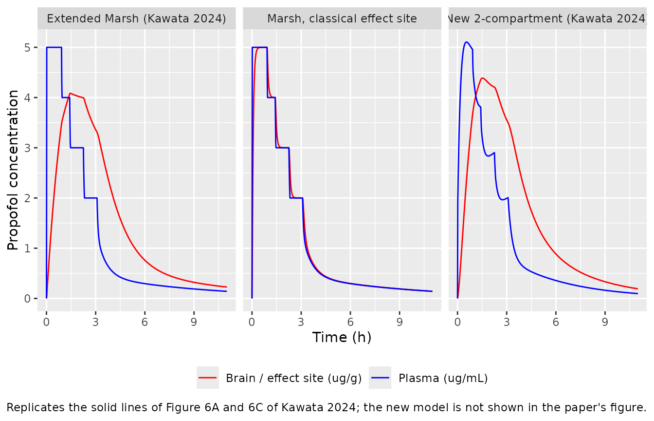
peak_marsh <- typ_marsh[which.max(typ_marsh$Cbrain), c("time", "Cbrain")]
peak_marsh
#>    time   Cbrain
#> 88   87 4.086103
plasma_at <- function(sim, t) sim$Cc[sim$time == t]
stopifnot(
  # The TCI controller holds the Marsh plasma concentration on target.
  abs(plasma_at(typ_marsh, 50) - 5) < 0.01,
  abs(plasma_at(typ_marsh, 120) - 3) < 0.01,
  abs(plasma_at(typ_marsh, 180) - 2) < 0.01,
  # Figure 6C: typical brain peak about 4.1 ug/g at about 1 h 20 min - 1 h 30 min
  # (read off the figure; the deterministic solve gives 4.09 ug/g at 87 min).
  abs(peak_marsh$Cbrain - 4.1) < 0.4,
  peak_marsh$time > 70,
  peak_marsh$time < 105
)
The extended Marsh model reproduces the shape of Figure 6C: the brain concentration lags the plasma concentration, peaks at 4.09 ug/g at 87 min, while the plasma target has already been lowered, and from then on stays above the plasma concentration. The classical effect site follows the plasma concentration within minutes, as in Figure 6A.
90% prediction interval (Figure 6C dashed lines)
n_sub <- 200L
ev_vpc <- make_events(seq_len(n_sub), schedule, seq(0, 660, by = 5), wt_typ)
rxode2::rxSetSeed(20240316)
sim_marsh <- rxode2::rxSolve(ui_marsh, events = ev_vpc, returnType = "data.frame")

pi_marsh <- sim_marsh |>
  dplyr::select(id, time, Cc, Cbrain) |>
  tidyr::pivot_longer(c(Cc, Cbrain), names_to = "output", values_to = "conc") |>
  dplyr::group_by(output, time) |>
  dplyr::summarise(
    q05 = quantile(conc, 0.05),
    q50 = quantile(conc, 0.50),
    q95 = quantile(conc, 0.95),
    .groups = "drop"
  )

ggplot(pi_marsh, aes(time / 60, q50, colour = output, fill = output)) +
  geom_ribbon(aes(ymin = q05, ymax = q95), alpha = 0.15, colour = NA) +
  geom_line() +
  scale_colour_manual(
    values = c(Cbrain = "red", Cc = "blue"),
    labels = c(Cbrain = "Brain (ug/g)", Cc = "Plasma (ug/mL)")
  ) +
  scale_fill_manual(
    values = c(Cbrain = "red", Cc = "blue"),
    labels = c(Cbrain = "Brain (ug/g)", Cc = "Plasma (ug/mL)")
  ) +
  labs(
    x = "Time (h)",
    y = "Propofol concentration",
    colour = NULL,
    fill = NULL,
    caption = "Extended Marsh model, 200 simulated patients: median and 90% interval of the individual predictions. Replicates Figure 6C of Kawata 2024."
  ) +
  theme(legend.position = "bottom")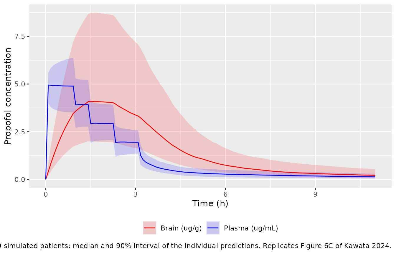
brain_90 <- dplyr::filter(pi_marsh, output == "Cbrain", time == 85)
plasma_50 <- dplyr::filter(pi_marsh, output == "Cc", time == 50)
dplyr::bind_rows(brain_90, plasma_50)
#> # A tibble: 2 × 5
#>   output  time   q05   q50   q95
#>   <chr>  <dbl> <dbl> <dbl> <dbl>
#> 1 Cbrain    85  2.00  4.07  8.67
#> 2 Cc        50  3.52  4.89  6.35
stopifnot(
  # Figure 6C at about 1 h 25 min: brain 90% interval about 2.0 to 8.2 ug/g.
  # Across three seeds at 1, 2 and 4 threads the 200-patient cohort gave a
  # brain 5th percentile of 1.71-2.16 and 95th of 7.10-8.67 ug/g, and a plasma
  # 5th of 3.43-3.60 and 95th of 6.35-6.53 ug/mL; the bounds sit outside that.
  brain_90$q05 > 1.2, brain_90$q05 < 3.0,
  brain_90$q95 > 6.0, brain_90$q95 < 11.0,
  # Figure 6C at about 50 min: plasma 90% interval about 3.5 to 6.5 ug/mL.
  plasma_50$q05 > 2.8, plasma_50$q05 < 4.4,
  plasma_50$q95 > 5.5, plasma_50$q95 < 8.0
)
Comparison with the observed concentrations after cessation
The supplement deposits every measured concentration, by time after the infusion was stopped, but not the infusion histories, so individual predictions cannot be recomputed. The table below sets the medians of the observed concentrations (all 57 patients, computed by the maintainers from the Supplementary dataset and binned by time after cessation) beside the typical-value predictions after the Figure 6 schedule, whose final plasma target of 2 ug/mL is close to the observed median of 2.2 ug/mL at cessation. The comparison is illustrative: the patients’ schedules differed from this one.
observed <- tibble::tribble(
  ~bin, ~t_after, ~n_pairs, ~plasma_obs, ~brain_obs, ~ratio_obs,
  "0 min", 0, 20, 2.21, 3.60, 1.60,
  "1-9 min", 5, 15, 1.53, 3.36, 2.25,
  "10-20 min", 15, 13, 0.99, 2.93, 2.79,
  "21-50 min", 33, 28, 0.91, 2.13, 2.22,
  "51-120 min", 82, 24, 0.44, 1.55, 3.56,
  "over 120 min", 152, 8, 0.29, 1.28, 5.29
)

pred_after <- function(sim, label) {
  sim |>
    dplyr::filter(time %in% (t_stop + observed$t_after)) |>
    dplyr::transmute(
      t_after = time - t_stop,
      model = label,
      plasma = Cc,
      brain = Cbrain,
      ratio = Cbrain / Cc
    )
}

pred <- dplyr::bind_rows(
  pred_after(typ_marsh, "marsh"),
  pred_after(typ_2cmt, "2cmt")
) |>
  tidyr::pivot_wider(
    names_from = model,
    values_from = c(plasma, brain, ratio)
  )

cmp_obs <- dplyr::left_join(observed, pred, by = "t_after")

cmp_obs |>
  dplyr::mutate(dplyr::across(where(is.double) & !c(t_after, n_pairs), ~ signif(.x, 3))) |>
  dplyr::select(
    bin,
    t_after,
    n_pairs,
    plasma_obs,
    plasma_marsh,
    plasma_2cmt,
    brain_obs,
    brain_marsh,
    brain_2cmt,
    ratio_obs,
    ratio_marsh,
    ratio_2cmt
  ) |>
  dplyr::rename(
    "Time bin" = bin,
    "Predicted at (min)" = t_after,
    "Paired samples" = n_pairs,
    "Plasma obs" = plasma_obs,
    "Plasma ext. Marsh" = plasma_marsh,
    "Plasma new" = plasma_2cmt,
    "Brain obs" = brain_obs,
    "Brain ext. Marsh" = brain_marsh,
    "Brain new" = brain_2cmt,
    "Ratio obs" = ratio_obs,
    "Ratio ext. Marsh" = ratio_marsh,
    "Ratio new" = ratio_2cmt
  ) |>
  knitr::kable(
    caption = "Median observed plasma (ug/mL) and brain (ug/g) concentrations and the median paired brain/plasma ratio, against typical-value predictions."
)| Time bin | Predicted at (min) | Paired samples | Plasma obs | Plasma ext. Marsh | Plasma new | Brain obs | Brain ext. Marsh | Brain new | Ratio obs | Ratio ext. Marsh | Ratio new |
|---|---|---|---|---|---|---|---|---|---|---|---|
| 0 min | 0 | 20 | 2.21 | 2.000 | 2.010 | 3.60 | 3.310 | 3.50 | 1.60 | 1.65 | 1.74 |
| 1-9 min | 5 | 15 | 1.53 | 1.300 | 1.640 | 3.36 | 3.220 | 3.43 | 2.25 | 2.48 | 2.09 |
| 10-20 min | 15 | 13 | 0.99 | 0.952 | 1.180 | 2.93 | 2.990 | 3.22 | 2.79 | 3.14 | 2.72 |
| 21-50 min | 33 | 28 | 0.91 | 0.710 | 0.807 | 2.13 | 2.560 | 2.78 | 2.22 | 3.60 | 3.44 |
| 51-120 min | 82 | 24 | 0.44 | 0.432 | 0.541 | 1.55 | 1.630 | 1.79 | 3.56 | 3.77 | 3.31 |
| over 120 min | 152 | 8 | 0.29 | 0.315 | 0.394 | 1.28 | 0.899 | 1.03 | 5.29 | 2.85 | 2.63 |
Both models reproduce what Figure 1C shows: the brain/plasma ratio is above 1 at cessation and rises as plasma falls faster than brain. Beyond 2 h after cessation the observed ratio (from only 8 paired samples) keeps rising while the predicted ratio levels off; the paper notes the same limitation, that a few high late brain concentrations may drive the late rise. The slow brain equilibration (k1e = 0.014 1/min, a half-life of about 50 min, against the classical ke0 of 0.26 1/min) is what keeps the brain concentration high after the infusion ends.
PKNCA validation
The paper reports no NCA. Because the brain compartment is linear, integrating its equation over the whole profile gives an exact identity: the brain AUC0-inf equals Kp times the plasma AUC0-inf for every patient. PKNCA is run on both outputs for 200 simulated patients per model, and the ratio of the two AUCs is compared with each patient’s own Kp.
ev_nca <- make_events(
  seq_len(n_sub),
  schedule,
  sort(unique(c(seq(0, 300, by = 5), seq(300, 1440, by = 20)))),
  wt_typ
)
rxode2::rxSetSeed(20240317)
sim_nca <- dplyr::bind_rows(
  rxode2::rxSolve(
    ui_marsh,
    events = ev_nca,
    returnType = "data.frame"
  ) |>
    dplyr::mutate(treatment = "Extended Marsh"),
  rxode2::rxSolve(
    ui_2cmt,
    events = ev_nca,
    returnType = "data.frame"
  ) |>
    dplyr::mutate(treatment = "New 2-compartment")
)
conc_long <- sim_nca |>
  dplyr::select(id, treatment, time, Cc, Cbrain) |>
  tidyr::pivot_longer(c(Cc, Cbrain), names_to = "analyte", values_to = "conc") |>
  dplyr::filter(!is.na(conc))
stopifnot(all(conc_long$conc >= -1e-6 * max(conc_long$conc)))
conc_long <- dplyr::mutate(conc_long, conc = pmax(conc, 0))

dose_df <- sim_nca |>
  dplyr::distinct(id, treatment) |>
  dplyr::mutate(time = 0, amt = sum(schedule$rate))

conc_obj <- PKNCA::PKNCAconc(conc_long, conc ~ time | treatment + id / analyte)
dose_obj <- PKNCA::PKNCAdose(dose_df, amt ~ time | treatment + id)
intervals <- data.frame(
  start = 0,
  end = Inf,
  cmax = TRUE,
  tmax = TRUE,
  aucinf.obs = TRUE,
  half.life = TRUE
)
nca_res <- PKNCA::pk.nca(PKNCA::PKNCAdata(conc_obj, dose_obj, intervals = intervals))

nca_tab <- as.data.frame(nca_res) |>
  dplyr::filter(PPTESTCD %in% c("cmax", "tmax", "aucinf.obs", "half.life"))

nca_tab |>
  dplyr::group_by(treatment, analyte, PPTESTCD) |>
  dplyr::summarise(median = signif(median(PPORRES, na.rm = TRUE), 3), .groups = "drop") |>
  tidyr::pivot_wider(names_from = PPTESTCD, values_from = median) |>
  dplyr::rename(
    "Model" = treatment,
    "Analyte" = analyte,
    "Cmax (ug/mL or ug/g)" = cmax,
    "Tmax (min)" = tmax,
    "AUC0-inf (ug*min/mL or ug*min/g)" = aucinf.obs,
    "t1/2 (min)" = half.life
  ) |>
knitr::kable(caption = "Median simulated NCA parameters after the Figure 6 schedule.")| Model | Analyte | AUC0-inf (ugmin/mL or ugmin/g) | Cmax (ug/mL or ug/g) | t1/2 (min) | Tmax (min) |
|---|---|---|---|---|---|
| Extended Marsh | Cbrain | 1100 | 3.92 | 292 | 90 |
| Extended Marsh | Cc | 860 | 4.90 | 293 | 5 |
| New 2-compartment | Cbrain | 1100 | 4.23 | 157 | 90 |
| New 2-compartment | Cc | 812 | 5.09 | 158 | 35 |
kp_ind <- sim_nca |>
  dplyr::distinct(treatment, id, kp_brain)

auc_ratio <- nca_tab |>
  dplyr::filter(PPTESTCD == "aucinf.obs") |>
  dplyr::select(treatment, id, analyte, PPORRES) |>
  tidyr::pivot_wider(names_from = analyte, values_from = PPORRES) |>
  dplyr::left_join(kp_ind, by = c("treatment", "id")) |>
  dplyr::mutate(pct_diff = 100 * (Cbrain / Cc / kp_brain - 1))

auc_ratio |>
  dplyr::group_by(treatment) |>
  dplyr::summarise(
    median_pct_diff = signif(median(pct_diff), 3),
    p90_abs_pct_diff = signif(quantile(abs(pct_diff), 0.9), 3),
    .groups = "drop"
  ) |>
  dplyr::rename(
    "Model" = treatment,
    "Median % difference" = median_pct_diff,
    "90th percentile |% difference|" = p90_abs_pct_diff
  ) |>
knitr::kable(caption = "Brain/plasma AUC0-inf ratio against each patient's Kp.")| Model | Median % difference | 90th percentile |% difference| |
|---|---|---|
| Extended Marsh | 0.692 | 0.878 |
| New 2-compartment | 0.306 | 0.372 |
stopifnot(
  nrow(auc_ratio) == 2 * n_sub,
  # A wrong brain equation (Kp on the output instead of the input, or ke0'
  # different from k1e) moves this by tens of percent. The residual is the
  # trapezoid and terminal-extrapolation error of the two AUCs.
  abs(median(auc_ratio$pct_diff)) < 3,
  quantile(abs(auc_ratio$pct_diff), 0.9) < 6
)
Assumptions and deviations
-
Brain state holds a concentration. In both control
streams the brain compartment is observed with no scale factor, so its
“amount” is the brain concentration (the paper takes brain tissue
density as 1 g/mL). The packaged
brainstate therefore holds ug/g, andCbrain <- brain. -
Parameter names. The paper’s k1e is encoded as
lke0(the canonical effect-compartment rate constant; the paper sets the brain elimination rate ke0’ equal to k1e) and Kp aslkp_brain. The Marsh micro-constants k10, k12, k13, k21, k31 arelkel,lk12,lk13,lk21,lk31, and the Marsh V1 of 0.228 L/kg islvcmultiplied byWT. - Variability scales. Tables 1 and 2 print interindividual variability as CV% and the additive brain error under a “Variance” heading. The new model’s control stream holds the final $OMEGA and $SIGMA values (0.0262, 0.148, 0.045, 0.772), and their square roots reproduce the printed 16.2%, 38.5%, 21.2% and 0.879 ug/g exactly, so the printed CV% is 100 x sqrt(omega^2) and the printed additive brain error is a standard deviation. The extended Marsh control stream carries only initial values (0.1), so its variances are taken from Table 1 on that same scale (omega^2 = (CV%/100)^2).
- Marsh k12. The paper fixes k12 at 0.114 1/min (Table 1 and Supplementary code 1), and the packaged model uses that value.
-
Unused volume statement. Supplementary code 1
computes
V3=Q2/k31(rather thanQ3/k31); V3 is not used by the differential equations or the observations, so it has no effect and is not carried over. - Full-data refit not packaged. Supplementary Table S3 refits the extended Marsh model to all 57 patients (k1e 0.0123 1/min, Kp 1.28) as a robustness check; the model-building fit of Table 1 is the reported final model.
- Figure 6 schedule. The TCI target step times (55, 85, 135 min) and the stop time (185 min) were read off Figure 6 by the maintainers, to about +/-5 min; the one-minute TCI controller is the maintainers’ reconstruction of a Marsh-driven pump, and the patient weight (62.5 kg) is the model-building median.
-
Covariates. The covariate screen (height, weight,
BMI, sex, AST, ALT, albumin, total bilirubin, creatinine) on Q4 = k1e x
V1 retained none; the screened covariates are listed under
covariatesDataExcluded. Ethnicity is not stated; all patients were enrolled at a single centre in Kyoto. - No correction notice for this article was found on Europe PMC as of 2026-10-29.