Palbociclib (Royer 2021)
Source:vignettes/articles/Royer_2021_palbociclib.Rmd
Royer_2021_palbociclib.RmdModel and source
Royer et al. (2021) built a population pharmacokinetic model of oral palbociclib from routine therapeutic drug monitoring samples in women treated for metastatic breast cancer at a French cancer centre. Most patients contributed a single plasma sample, drawn at a follow-up visit with no constraint on the time after dose or on the day of the cycle. The final model is one-compartment with first-order absorption, an absorption lag time fixed to an earlier analysis, and first-order elimination. Apparent clearance increases with Cockcroft-Gault creatinine clearance (CRCL).
- Article: https://doi.org/10.3390/ph14030181 (open access)
mod <- rxode2::rxode(readModelDb("Royer_2021_palbociclib"))
#> ℹ parameter labels from comments will be replaced by 'label()'- Citation: Royer B, Kaderbhai C, Fumet JD, Hennequin A, Desmoulins I, Ladoire S, Ayati S, Mayeur D, Ilie S, Schmitt A. (2021). Population Pharmacokinetics of Palbociclib in a Real-World Situation. Pharmaceuticals 14(3):181. doi:10.3390/ph14030181.
- Description: One-compartment population PK model with first-order absorption, a fixed absorption lag time and first-order elimination for oral palbociclib in women with metastatic breast cancer followed in routine care (therapeutic drug monitoring, mostly one sample per patient). Apparent oral clearance increases with Cockcroft-Gault creatinine clearance through a power model centred on the cohort mean of 78.9 mL/min (exponent 0.419). Correlated inter-individual variability on CL/F and ka; combined additive + proportional residual error.
Population
The analysis used 151 plasma concentrations from 124 women (Results, section 2), sampled between 28 October 2018 and 3 August 2020. Twenty-seven patients had two samples; for 25 of them the two samples came from different cycles and the authors modelled them as independent individuals, so no inter-occasion variability was estimated. Patients received 75 mg (n = 15), 100 mg (n = 33) or 125 mg (n = 101) once daily on the usual 21-days-on / 7-days-off schedule, with an aromatase inhibitor or fulvestrant. Table 1 gives age 40.7-92.2 years (mean 67.4), body weight 37-140 kg (mean 69.7) and Cockcroft-Gault CRCL 23.4-282.3 mL/min (mean 78.9, median 72.1). Samples were drawn 0.9-197.25 h after the previous dose; concentrations ranged 6-226 ug/L with a mean of 81.8 ug/L.
Source trace
| Element | Value | Source |
|---|---|---|
| Structure: 1-compartment, first-order absorption, lag time, combined error | – | Results section 2, first paragraph after Table 1 reference |
lka |
log(0.187 /h) | Table 2, Ka |
lcl |
log(58.3 L/h) | Table 2, CL/F |
lvc |
log(1580 L) | Table 2, V/F |
ltlag |
fixed(log(0.658 h)) | Table 2, Tlag; fixed to reference 7 (Sun and Wang 2014) per Results section 2 |
e_crcl_cl |
0.419 | Table 2, CRCL on CL/F |
| CRCL centring value | 78.9 mL/min | Section 4.3 (power model normalized to the population mean) and Table 1 (mean CRCL) |
etalcl variance |
log(1 + 0.313^2) = 0.09346 | Table 2, IIV CL/F 31.3% |
etalka variance |
log(1 + 1.261^2) = 0.95170 | Table 2, IIV Ka 126.1% |
etalcl-etalka covariance |
-0.342 x sqrt(0.09346 x 0.95170) = -0.10200 | Table 2, correlation between CL/F and Ka -34.2% |
addSd |
8.14 ug/L | Table 2, Additional Error |
propSd |
0.0689 | Table 2, Proportional Error |
Cc <- 1000 * central / vc |
mg/L to ug/L | Units of Table 2 and section 4.2 |
Steady-state typical profiles
The typical patient (CRCL = 78.9 mL/min, all random effects zero) receives each of the three doses once daily for 21 days. The last dosing interval (480-504 h) is sampled densely.
doses <- c(75, 100, 125)
tau <- 24
obs_grid <- sort(unique(c(seq(0, 480, by = 12), 480 + seq(0, 24, by = 0.25))))

ev_ss <- lapply(seq_along(doses), function(i) {
  rxode2::et(amt = doses[[i]], cmt = "depot", ii = tau, addl = 20) |>
    rxode2::et(obs_grid, cmt = "central") |>
    as.data.frame() |>
    dplyr::mutate(id = i)
}) |>
  dplyr::bind_rows() |>
  dplyr::mutate(CRCL = 78.9)

sim_ss <- rxode2::rxSolve(
  rxode2::zeroRe(mod),
  events = ev_ss,
  rtol = 1e-10, atol = 1e-12,
  returnType = "data.frame"
) |>
  dplyr::mutate(dose = doses[id], treatment = paste(dose, "mg QD"))
#> ℹ omega/sigma items treated as zero: 'etalcl', 'etalka'
#> Warning: multi-subject simulation without without 'omega'
ggplot(sim_ss, aes(time / 24, Cc, colour = treatment)) +
  geom_line() +
  labs(x = "Day of cycle", y = "Palbociclib (ug/L)", colour = NULL) +
  theme_bw()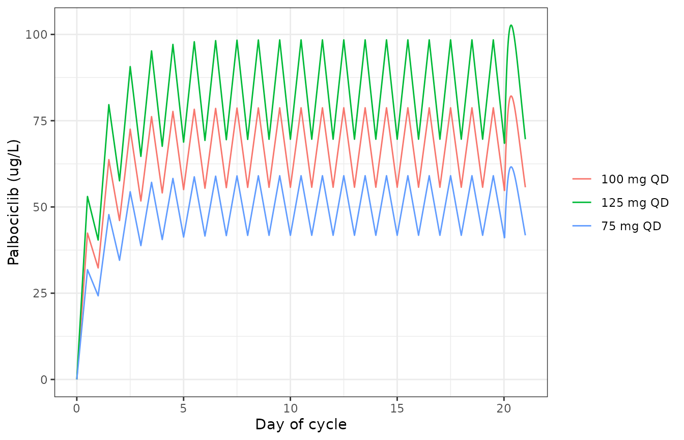
Typical palbociclib concentration over the 21 days of a cycle (CRCL = 78.9 mL/min).
Closed-form check
With the lag time the dosing interval is shifted by
tlag, so the steady-state one-compartment solution is
evaluated at (t - tlag) %% tau. After 21 doses the
non-steady-state remainder is exp(-kel * 480), about 2e-8,
so the solve and the formula must agree to far better than 1e-6.
p <- list(ka = 0.187, cl = 58.3, vc = 1580, tlag = 0.658)
kel <- p$cl / p$vc
css <- function(t, dose) {
  tp <- (t - p$tlag) %% tau
  1000 * dose * p$ka / (p$vc * (p$ka - kel)) *
    (exp(-kel * tp) / (1 - exp(-kel * tau)) - exp(-p$ka * tp) / (1 - exp(-p$ka * tau)))
}
last_int <- sim_ss |>
  dplyr::filter(time >= 480 + p$tlag + 0.1, time <= 504) |>
  dplyr::mutate(Cc_cf = css(time, dose))
rel_err <- max(abs(last_int$Cc / last_int$Cc_cf - 1))
rel_err
#> [1] 1.927137e-08
stopifnot(rel_err < 1e-6)
NCA over the last dosing interval (PKNCA)
conc_ss <- sim_ss |>
  dplyr::filter(!is.na(Cc), time >= 480, time <= 504) |>
  dplyr::mutate(time = time - 480, Cc = pmax(Cc, 0)) |>
  dplyr::select(id, treatment, time, Cc)
dose_ss <- data.frame(id = seq_along(doses), treatment = paste(doses, "mg QD"), time = 0, amt = doses)

conc_obj <- PKNCA::PKNCAconc(conc_ss, Cc ~ time | treatment + id, concu = "ug/L", timeu = "h")
dose_obj <- PKNCA::PKNCAdose(dose_ss, amt ~ time | treatment + id, doseu = "mg")
intervals <- data.frame(
  start = 0, end = 24,
  cmax = TRUE, tmax = TRUE, cmin = TRUE, auclast = TRUE, cav = TRUE
)
nca_res <- PKNCA::pk.nca(PKNCA::PKNCAdata(conc_obj, dose_obj, intervals = intervals))
nca_wide <- as.data.frame(nca_res$result) |>
  dplyr::select(treatment, PPTESTCD, PPORRES) |>
  tidyr::pivot_wider(names_from = PPTESTCD, values_from = PPORRES)

nca_wide |>
  dplyr::mutate(auc_closed = 1000 * as.numeric(sub(" mg QD", "", treatment)) / p$cl) |>
  dplyr::rename(
    "Dose" = treatment,
    "Cmax,ss (ug/L)" = cmax,
    "Tmax (h)" = tmax,
    "Cmin,ss (ug/L)" = cmin,
    "AUC0-24,ss (ug*h/L)" = auclast,
    "Cavg,ss (ug/L)" = cav,
    "Dose/CL (ug*h/L)" = auc_closed
  ) |>
knitr::kable(digits = 1, caption = "Typical-value steady-state NCA on day 21 (CRCL = 78.9 mL/min).")| Dose | AUC0-24,ss (ug*h/L) | Cmax,ss (ug/L) | Cmin,ss (ug/L) | Tmax (h) | Cavg,ss (ug/L) | Dose/CL (ug*h/L) |
|---|---|---|---|---|---|---|
| 100 mg QD | 1715.3 | 82.2 | 54.8 | 8 | 71.5 | 1715.3 |
| 125 mg QD | 2144.1 | 102.7 | 68.4 | 8 | 89.3 | 2144.1 |
| 75 mg QD | 1286.5 | 61.6 | 41.1 | 8 | 53.6 | 1286.4 |
# PKNCA sorts the groups by label, so recover each row's dose from its label.
auc_ratio <- nca_wide$auclast / (1000 * as.numeric(sub(" mg QD", "", nca_wide$treatment)) / p$cl)
auc_ratio
#> [1] 1.000012 1.000012 1.000012
# The trapezoid on a 0.25-h grid differs from the exact Dose/CL by well under 1%;
# a wrong clearance, dose or unit factor moves it by tens of percent.
stopifnot(all(abs(auc_ratio - 1) < 0.01))
Royer 2021 reports no NCA table, so there is no published NCA to
compare against. The model’s typical half-life is
log(2) * V/F / (CL/F) = 18.8 h, shorter than the 29 h
reported in the product label that the paper cites (reference 2). The
authors note in the Discussion that their sparse, mostly single-sample
design could support only a one-compartment model, whereas the earlier
analysis with rich sampling was two-compartment.
Dose-weighted average concentration
The Results report a mean observed concentration of 81.8 ug/L. The typical steady-state average concentration weighted by the dose counts the paper gives (15 x 75 mg, 33 x 100 mg, 101 x 125 mg) reproduces it:
n_dose <- c(15, 33, 101)
cavg_weighted <- sum(n_dose * 1000 * doses / (p$cl * tau)) / sum(n_dose)
cavg_weighted
#> [1] 81.78211
stopifnot(abs(cavg_weighted / 81.8 - 1) < 0.05)
This is a consistency check of CL/F against the data summary, not an exact identity: individual clearances vary, and 20% of samples were drawn in the first 8 days of a cycle, before steady state.
Effect of creatinine clearance on CL/F
Replicates the covariate relationship shown in Figure 2 of Royer
2021: CL/F is proportional to (CRCL / 78.9)^0.419.
crcl_grid <- data.frame(CRCL = seq(23.4, 282.3, length.out = 200)) |>
  dplyr::mutate(cl = 58.3 * (CRCL / 78.9)^0.419)
ggplot(crcl_grid, aes(CRCL, cl)) +
  geom_line() +
  geom_vline(xintercept = 78.9, linetype = 2) +
  labs(x = "Cockcroft-Gault CRCL (mL/min)", y = "Typical CL/F (L/h)") +
  theme_bw()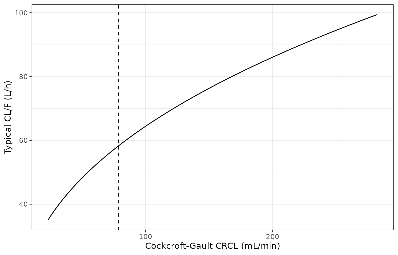
Typical CL/F across the observed CRCL range (23.4-282.3 mL/min).
cl_at <- function(crcl) 58.3 * (crcl / 78.9)^0.419
auc_increase <- c(
  mild = cl_at(90) / cl_at(75) - 1,
  moderate = cl_at(90) / cl_at(45) - 1,
  severe = cl_at(90) / cl_at(20) - 1
)
round(100 * auc_increase, 1)
#>     mild moderate   severe
#>      7.9     33.7     87.8
Relative to a patient with CRCL = 90 mL/min, the model predicts steady-state exposure (Dose / CL/F) higher by the percentages above at CRCL of 75, 45 and 20 mL/min. The Discussion compares this direction of effect with a dedicated renal-impairment study (reference 5: AUC increases of 31%, 45% and 57% for mild, moderate and severe impairment); that study used a different population and is shown here for context only, not as a validation target.
Simulated sparse-sampling cohort
Replicates the layout of Figure 3D of Royer 2021: one concentration per patient, drawn at a random time within the 21 dosing days of a cycle. Each virtual patient receives 75, 100 or 125 mg in the paper’s proportions, and CRCL is drawn from a log-normal with the Table 1 median (72.1 mL/min) and mean (78.9 mL/min), redrawn until it falls within the observed 23.4-282.3 mL/min range. The sample is taken 1-24 h after the dose on a day drawn uniformly from days 1-21; the paper states only that most samples were drawn within 36 h of a dose.
rxode2::rxSetSeed(20210224)
set.seed(20210224)
n_sub <- 200

draw_crcl <- function(n) {
  sdlog <- sqrt(2 * log(78.9 / 72.1))
  out <- numeric(0)
  while (length(out) < n) {
    x <- rlnorm(n, log(72.1), sdlog)
    out <- c(out, x[x >= 23.4 & x <= 282.3])
  }
  out[seq_len(n)]
}

cohort <- data.frame(
  id = seq_len(n_sub),
  dose = sample(doses, n_sub, replace = TRUE, prob = n_dose / sum(n_dose)),
  CRCL = draw_crcl(n_sub),
  day = sample(1:21, n_sub, replace = TRUE),
  tad = runif(n_sub, 1, 24)
) |>
  dplyr::mutate(tsamp = (day - 1) * 24 + tad)

dose_rows <- cohort |>
  dplyr::select(id, dose, CRCL) |>
  dplyr::slice(rep(seq_len(n_sub), each = 21)) |>
  dplyr::group_by(id) |>
  dplyr::mutate(time = (dplyr::row_number() - 1) * 24) |>
  dplyr::ungroup() |>
  dplyr::transmute(id, time, amt = dose, evid = 1L, cmt = "depot", CRCL)
obs_rows <- cohort |>
  dplyr::transmute(id, time = tsamp, amt = 0, evid = 0L, cmt = "central", CRCL)
ev_cohort <- dplyr::bind_rows(dose_rows, obs_rows) |>
  dplyr::arrange(id, time, dplyr::desc(evid))

sim_cohort <- rxode2::rxSolve(mod, events = ev_cohort, returnType = "data.frame") |>
  dplyr::left_join(cohort |> dplyr::select(id, dose), by = "id")
ggplot(sim_cohort, aes(time, sim)) +
  geom_point(aes(colour = factor(dose)), alpha = 0.6) +
  geom_smooth(method = "loess", formula = y ~ x, se = FALSE, colour = "black") +
  labs(x = "Time since start of cycle (h)", y = "Palbociclib (ug/L)", colour = "Dose (mg)") +
  theme_bw()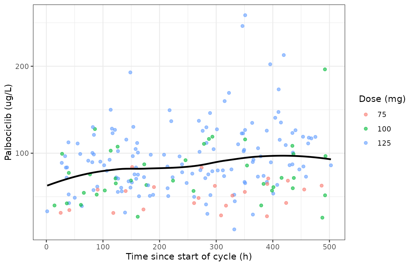
Simulated single samples versus time since the start of the cycle (compare Figure 3D of Royer 2021, which shows observed concentrations mostly between 25 and 200 ug/L with a median near 80-90 ug/L).
summary(sim_cohort$sim)
#>    Min. 1st Qu.  Median    Mean 3rd Qu.    Max.
#>   12.37   59.73   80.91   86.86  109.57  258.69
# Centre of the simulated single samples against the reported mean of 81.8 ug/L.
# A mis-transcribed clearance, dose or unit moves this by tens of percent; the
# standard error of a 200-subject mean at ~40% CV is about 3%.
stopifnot(abs(mean(sim_cohort$sim) / 81.8 - 1) < 0.2)
Assumptions and deviations
-
IIV scale. Table 2 prints IIV as percentages (31.3%
on CL/F, 126.1% on Ka) without stating the conversion. They are read as
coefficients of variation and converted with
omega^2 = log(1 + CV^2). If the authors instead printed100 * sqrt(omega^2), the variances would be 0.0980 (CL/F) and 1.590 (Ka). The CL/F difference is negligible; the Ka difference is large, but Ka IIV had 63.5% shrinkage and drives only the absorption phase. -
Residual error scale. The additive error carries a
ug/L unit in Table 2 and is read as a standard deviation. The
proportional error (0.0689) is also read as a standard deviation (a 6.9%
proportional component); the table does not say whether it is a standard
deviation or a variance. The combined model is encoded as nlmixr2’s
default
add() + prop()form, with the two components combined in variance. - Tlag unit. Table 2 labels Tlag as “(L)”; it is a time in hours, fixed to the value of an earlier analysis (Sun and Wang 2014, reference 7).
- CRCL centring. Section 4.3 states that continuous covariates were normalized by the population mean; the Table 1 mean CRCL of 78.9 mL/min is used. CRCL is the raw Cockcroft-Gault value in mL/min, not BSA-normalized.
- Table 1 body-weight median. Table 1 prints a median weight of 98.0 kg against a mean of 69.7 kg, which is not plausible; body weight is not in the final model.
- Simulated sampling design. The paper does not tabulate sampling days or times after dose. The virtual cohort draws the day of the cycle uniformly over days 1-21 and the time after dose uniformly over 1-24 h.
- Race / ethnicity were not reported.