Li_2019_abatacept

Model and source

Citation: Li X, Roy A, Murthy B. Population Pharmacokinetics and Exposure-Response Relationship of Intravenous and Subcutaneous Abatacept in Patients With Rheumatoid Arthritis. J Clin Pharmacol. 2019 Feb;59(2):245-257. doi:10.1002/jcph.1308
Description: Two-compartment population PK model for abatacept (CTLA4-Ig Fc-fusion) in adults with rheumatoid arthritis (Li 2019), with first-order SC absorption, zero-order IV infusion support, first-order linear elimination, logit-scale SC bioavailability, full-block IIV on CL/VC/Q/VP, and a KA parameterisation that enforces KA > k_el.
Article: J Clin Pharmacol. 2019;59(2):245-257 (open access via PMC6587803)

Population

Li 2019 pooled 11 clinical studies (4 phase 2 and 7 phase 3) into a final population PK dataset of 2244 adults with rheumatoid arthritis (RA). Six studies administered IV abatacept, four studies administered SC abatacept, and one study (ACQUIRE) investigated both routes. Doses ranged from 0.5 to 10 mg/kg Q4W for IV administration and 75 to 200 mg QW for SC administration. After exclusion of samples missing dose/sample information and below-LLOQ concentrations, the analysis dataset contained 10,382 measurements (validated ELISA, LLOQ 1.0 ng/mL).

The approved regimens are a weight-tiered ~10 mg/kg IV Q4W (500 mg for <60 kg, 750 mg for 60-100 kg, 1000 mg for >100 kg) and a fixed 125 mg SC QW. Li 2019 concluded that both regimens are comparable, delivering steady-state trough concentration (C_minss) ≥10 μg/mL — the exposure target associated with near-maximal DAS28 response — in ~90% of patients across all body weight strata.

The same information is available programmatically via readModelDb("Li_2019_abatacept")$population.

Source trace

Every structural parameter, covariate effect, IIV element, and residual-error term below is taken from Li 2019 Table 1 (A: final-model structural parameters, B: covariate effects; see also the Errata section for Table 1B’s caption issue). Reference covariate values are: 50-year-old male, baseline body weight 70 kg, baseline albumin 4.0 g/dL (paper typo: “mg/dL”), calculated GFR 90 mL/min/1.73 m², swollen joint count 16, not on concomitant NSAIDs, treated with the phase-3 (commercial) SC formulation.

Equation / parameter	Value	Source location
`lcl` (CL)	`log(0.0204 * 24)` L/day	Table 1A, CL_TV,ref = 0.0204 L/h
`lvc` (VC)	`log(3.27)` L	Table 1A, VC_TV,ref = 3.27 L
`lq` (Q)	`log(0.0265 * 24)` L/day	Table 1A, Q_TV,ref = 0.0265 L/h
`lvp` (VP)	`log(4.26)` L	Table 1A, VP_TV,ref = 4.26 L
`lka` (KA_TV)	`log(0.00305 * 24)` 1/day	Table 1A, KA_TV = 0.00305 1/h
`logitfdepot` (logit F_TV,ref)	`1.42`	Table 1A, SC F_TV,ref = 1.42 (logit scale)
`e_wt_cl` ((WT/70)^exp on CL)	`0.651`	Table 1B, CL_BWT = 0.651
`e_wt_vc` ((WT/70)^exp on VC)	`0.452`	Table 1B, VC_BWT = 0.452
`e_wt_vp` ((WT/70)^exp on VP)	`0.457`	Table 1B, VP_BWT = 0.457
`e_age_cl` ((AGE/50)^exp on CL)	`-0.186`	Table 1B, CL_AGE = -0.186
`e_alb_cl` ((ALB/4.0)^exp on CL)	`-0.687`	Table 1B, CL_ALB = -0.687
`e_crcl_cl` ((CRCL/90)^exp on CL)	`0.162`	Table 1B, CL_cGFR = 0.162
`e_swol_cl` (((SWOL+1)/17)^exp on CL)	`0.0965`	Table 1B, CL_SWOL = 0.0965
`e_sexf_cl` (exp(SEXF·coef) on CL)	`-0.0722`	Table 1B, CL_SEX = -0.0722
`e_nsaid_cl` (exp(CONMED_NSAID·coef) on CL)	`0.0640`	Table 1B, CL_NSAID = 0.0640
`e_form_f` (+coef·FORM on logit-F)	`-1.16`	Table 1B, F_FORM = -1.16
`var(etalcl)`	`0.0991`	Table 1A, var(ZCL)
`var(etalvc)`	`0.0632`	Table 1A, var(ZVC)
`var(etalq)`	`0.429`	Table 1A, var(ZQ)
`var(etalvp)`	`0.377`	Table 1A, var(ZVP)
`var(etalka)`	`1.63`	Table 1A, var(ZKA)
`var(etalogitfdepot)`	`0.710`	Table 1A, var(ZF) (logit scale)
`cov(etalcl, etalvc)`	`0.0412`	Table 1A, ZCL:ZVC
`cov(etalcl, etalq)`	`0.0952`	Table 1A, ZCL:ZQ
`cov(etalcl, etalvp)`	`0.0910`	Table 1A, ZCL:ZVP
`cov(etalvc, etalq)`	`0.0407`	Table 1A, ZVC:ZQ
`cov(etalvc, etalvp)`	`0.0675`	Table 1A, ZVC:ZVP
`cov(etalq, etalvp)`	`0.280`	Table 1A, ZQ:ZVP
`propSd`	`0.215`	Table 1A, θ_PROP = 0.215
`addSd`	`0.341` mg/L	Table 1A, θ_ADD = 0.341 μg/mL
Structure (2-cmt + first-order SC / zero-order IV input + logit-F + KA > k_el constraint + combined residual error)	n/a	Methods p. 247 (PopPK Analysis); Results p. 249 (final-model covariate equations)

Parameterization notes

Time-unit conversion. Li 2019 reports CL and Q in L/h and KA in 1/h. The nlmixr2lib convention is time in days, so each of these values is multiplied by 24 inside log(...) in ini().
Logit-F parameterisation. Li 2019 constrains absolute bioavailability to (0, 1) via an inverse-logit link: F_abs = 1 / (1 + exp(-F_TV)) with F_TV = logitfdepot + etalogitfdepot + FORM_ABA_PHASE2 * e_form_f. The reference value logitfdepot = 1.42 gives F_abs ~= 0.805 for the phase-3 commercial formulation; the phase-2 formulation shifts F_TV by -1.16, giving F_abs ~= 0.565.
KA > k_el constraint. Li 2019 reports a ~4-day SC Tmax and a ~14-day terminal half-life — i.e. absorption is faster than elimination. To prevent flip-flop of parameter estimates during fitting, the paper reparameterises absorption as KA_i = KA_TV * exp(etaKA) + k_el,i with k_el,i = CL_i / VC_i. The model file implements this verbatim; a simulation using only the typical parameters reproduces a Tmax of approximately 4.5 days (see below).
Full-block IIV on CL, VC, Q, VP. Li 2019 fits a 4×4 block covariance matrix on the CL, VC, Q, VP etas; the 10 lower-triangle values are taken directly from Table 1A. IIV on KA and on logit-F are independent blocks.
Combined proportional + additive residual error. Li 2019 reports θ_PROP = 0.215 (fraction) and θ_ADD = 0.341 μg/mL; nlmixr2lib uses mg/L for concentration, so addSd = 0.341 carries through without conversion (1 μg/mL = 1 mg/L).
SWOL shifted-power form. The swollen-joint-count effect is ((SWOL+1)/(16+1))^0.0965; adding 1 avoids the zero-count edge case at the origin of the power form.
Canonical CRCL usage. Li 2019 calls the renal covariate cGFR with units mL/min/1.73 m²; the canonical CRCL column carries the same units and accepts either an MDRD-estimated eGFR or a BSA-normalised measured CrCl. Reference 90.
MTX dropped by backward elimination. Table 1B lists a CL_MTX row (-0.0405, 95% CI -0.0889 to 0.00791, not significant) but the paper’s final-model covariate equation on p. 249 does not include an MTX term. This model implements the published equation and therefore excludes MTX; see Errata.

Virtual cohort

The simulations below use a virtual cohort whose covariate distributions approximate the Li 2019 Methods baseline-demographic descriptors (Table S3 is not accessible in the PMC full text). Subject-level observed data were not released with the paper.

set.seed(20260424)
n_subj <- 400

cohort <- tibble::tibble(
  id              = seq_len(n_subj),
  WT              = pmin(pmax(rnorm(n_subj, mean = 70, sd = 18),   40, 160)),
  AGE             = pmin(pmax(rnorm(n_subj, mean = 50, sd = 13),   18,  90)),
  ALB             = pmin(pmax(rnorm(n_subj, mean = 4.0, sd = 0.35), 2.5, 5.0)),
  CRCL            = pmin(pmax(rnorm(n_subj, mean = 90, sd = 25),   30, 180)),
  SWOL_28JOINT    = pmin(pmax(round(rnorm(n_subj, mean = 16, sd = 6)),   0,  28)),
  SEXF            = rbinom(n_subj, 1, 0.78),         # RA populations are ~75-80% female
  CONMED_NSAID    = rbinom(n_subj, 1, 0.55),         # Li 2019 Methods: NSAID use common in RA cohort
  FORM_ABA_PHASE2 = 0L                               # Phase-3 commercial SC formulation for labelled regimen
)

Three regimens are simulated: the labelled 125 mg SC QW (reference); weight-tiered IV Q4W (500 mg if <60 kg, 750 mg if 60-100 kg, 1000 mg if >100 kg); and a single-dose 125 mg SC for the Tmax / Cmax check.

tau_sc <- 7         # SC QW
tau_iv <- 28        # IV Q4W
n_sc   <- 26        # 26 weekly doses -> ~182 days, deeply into SS
n_iv   <- 7         # 7 q4w doses -> ~196 days

dose_days_sc <- seq(0, tau_sc * (n_sc - 1), by = tau_sc)
dose_days_iv <- seq(0, tau_iv * (n_iv - 1), by = tau_iv)

# Weight-tiered IV amount per subject
cohort_iv <- cohort |>
  dplyr::mutate(
    amt_iv = dplyr::case_when(
      WT <  60             ~ 500,
      WT <= 100            ~ 750,
      TRUE                 ~ 1000
    )
  )

build_sc_events <- function(cohort, dose_amt, dose_days, treatment) {
  ev_dose <- cohort |>
    tidyr::crossing(time = dose_days) |>
    dplyr::mutate(amt = dose_amt, cmt = "depot", evid = 1L, treatment = treatment)
  obs_days <- sort(unique(c(
    seq(0, max(dose_days) + tau_sc, by = 1),
    dose_days + 1, dose_days + 3
  )))
  ev_obs <- cohort |>
    tidyr::crossing(time = obs_days) |>
    dplyr::mutate(amt = 0, cmt = NA_character_, evid = 0L, treatment = treatment)
  dplyr::bind_rows(ev_dose, ev_obs) |>
    dplyr::arrange(id, time, dplyr::desc(evid))
}

build_iv_events <- function(cohort_iv, dose_days, treatment) {
  ev_dose <- cohort_iv |>
    tidyr::crossing(time = dose_days) |>
    dplyr::mutate(amt = amt_iv, cmt = "central", evid = 1L, treatment = treatment)
  obs_days <- sort(unique(c(
    seq(0, max(dose_days) + tau_iv, by = 1),
    dose_days + 1, dose_days + 7
  )))
  ev_obs <- cohort_iv |>
    tidyr::crossing(time = obs_days) |>
    dplyr::mutate(amt = 0, cmt = NA_character_, evid = 0L, treatment = treatment)
  dplyr::bind_rows(ev_dose, ev_obs) |>
    dplyr::arrange(id, time, dplyr::desc(evid))
}

events_sc_125 <- build_sc_events(cohort, 125, dose_days_sc, "SC_125_QW")
events_iv     <- build_iv_events(cohort_iv, dose_days_iv, "IV_weight_tiered_Q4W")

Simulation

mod <- rxode2::rxode2(readModelDb("Li_2019_abatacept"))
keep_cols <- c("WT", "AGE", "ALB", "CRCL", "SWOL_28JOINT",
               "SEXF", "CONMED_NSAID", "FORM_ABA_PHASE2", "treatment")

sim_sc <- as.data.frame(rxode2::rxSolve(mod, events = events_sc_125, keep = keep_cols))
sim_iv <- as.data.frame(rxode2::rxSolve(mod, events = events_iv,     keep = keep_cols))
sim    <- dplyr::bind_rows(sim_sc, sim_iv)

Replicate published figures

SC absorption: Tmax and early-dose kinetics

Li 2019 narrates “the time to maximum concentration (Tmax) for SC abatacept was ~4 days and the terminal half-life was ~14 days for both IV and SC abatacept.” The block below confirms the model reproduces that Tmax by simulating a single 125 mg SC dose at typical covariate values and plotting the concentration-time profile over 28 days.

mod_typ <- mod |> rxode2::zeroRe()
typ_cov <- tibble::tibble(
  id = 1L, WT = 70, AGE = 50, ALB = 4.0, CRCL = 90,
  SWOL_28JOINT = 16, SEXF = 0L, CONMED_NSAID = 0L, FORM_ABA_PHASE2 = 0L
)
ev_single_sc <- typ_cov |>
  tidyr::crossing(time = c(0, seq(0.25, 28, by = 0.25))) |>
  dplyr::mutate(amt = ifelse(time == 0, 125, 0),
                cmt = ifelse(time == 0, "depot", NA_character_),
                evid = ifelse(time == 0, 1L, 0L)) |>
  dplyr::arrange(id, time, dplyr::desc(evid))
sim_single_sc <- as.data.frame(rxode2::rxSolve(mod_typ, events = ev_single_sc))
#> ℹ omega/sigma items treated as zero: 'etalcl', 'etalvc', 'etalq', 'etalvp', 'etalka', 'etalogitfdepot'

tmax_day  <- sim_single_sc$time[which.max(sim_single_sc$Cc)]
cmax_mgL  <- max(sim_single_sc$Cc)

ggplot(sim_single_sc, aes(time, Cc)) +
  geom_line(linewidth = 0.8) +
  geom_vline(xintercept = tmax_day, linetype = "dashed", colour = "steelblue") +
  labs(
    x = "Time after single SC dose (days)",
    y = "Abatacept Cc (mg/L = µg/mL)",
    title = sprintf("Typical-patient single 125 mg SC: Tmax = %.1f days, Cmax = %.2f mg/L",
                    tmax_day, cmax_mgL),
    caption = "Li 2019 narrates 'Tmax for SC abatacept was ~4 days'."
  ) +
  theme_minimal()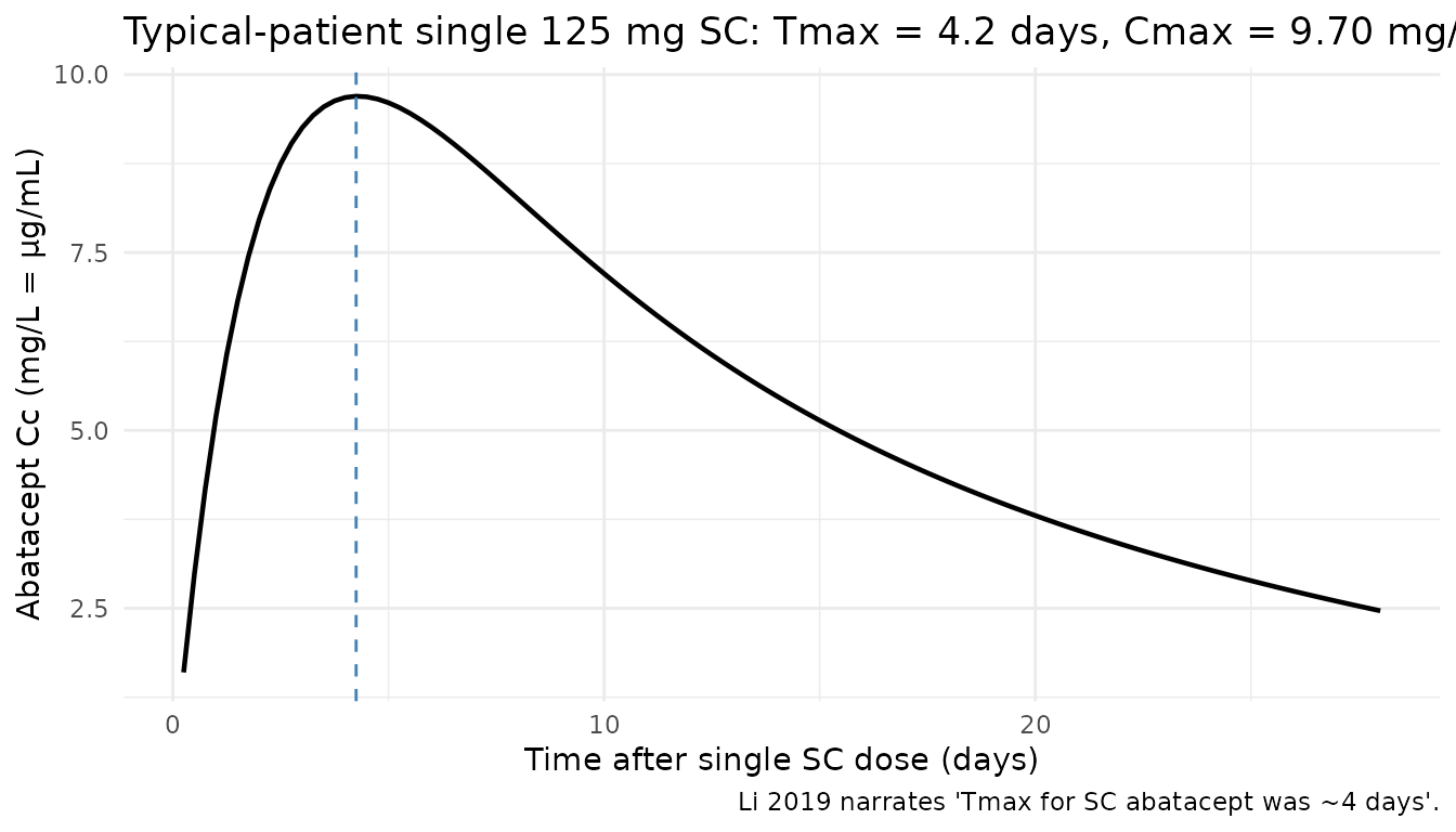

Concentration-time profiles: SC QW vs IV Q4W

The two approved regimens are overlaid on the same axes over the first 12 weeks. Percentile bands reflect cohort-level IIV.

vpc <- sim |>
  dplyr::filter(!is.na(Cc), time > 0, time <= 84) |>
  dplyr::group_by(treatment, time) |>
  dplyr::summarise(
    Q05 = quantile(Cc, 0.05, na.rm = TRUE),
    Q50 = quantile(Cc, 0.50, na.rm = TRUE),
    Q95 = quantile(Cc, 0.95, na.rm = TRUE),
    .groups = "drop"
  )

ggplot(vpc, aes(time, Q50, colour = treatment, fill = treatment)) +
  geom_ribbon(aes(ymin = Q05, ymax = Q95), alpha = 0.2, colour = NA) +
  geom_line(linewidth = 0.8) +
  labs(
    x = "Time (days)",
    y = "Abatacept Cc (mg/L)",
    title = "Simulated 5-50-95 percentile profiles: 125 mg SC QW vs weight-tiered ~10 mg/kg IV Q4W",
    caption = "Virtual RA cohort (N = 400); first 12 weeks."
  ) +
  theme_minimal()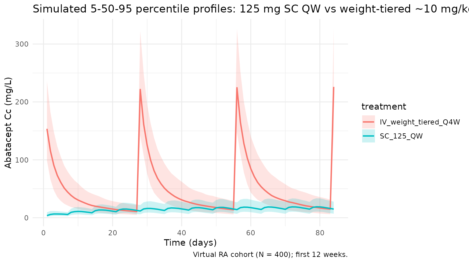

Steady-state exposures by body-weight group (Figure S2 replication)

Li 2019 Figure S2 plots simulated steady-state trough (C_minss) by body weight group (<60 kg, 60-100 kg, >100 kg) for IV and SC treatments and shows that (a) SC C_minss decreases with increasing body weight while (b) IV C_minss is approximately constant across weight groups by virtue of the weight-tiered dosing. The block below replicates that body-weight-group summary using the steady-state cycle of the virtual cohort.

ss_start_sc <- tau_sc * (n_sc - 1)
ss_end_sc   <- ss_start_sc + tau_sc
ss_start_iv <- tau_iv * (n_iv - 1)
ss_end_iv   <- ss_start_iv + tau_iv

trough_by_wtgrp <- dplyr::bind_rows(
  sim_sc |>
    dplyr::filter(time == ss_start_sc + tau_sc) |>
    dplyr::mutate(regimen = "SC 125 mg QW"),
  sim_iv |>
    dplyr::filter(time == ss_start_iv + tau_iv) |>
    dplyr::mutate(regimen = "IV weight-tiered Q4W")
) |>
  dplyr::mutate(
    wt_group = cut(WT, breaks = c(-Inf, 60, 100, Inf),
                   labels = c("<60 kg", "60-100 kg", ">100 kg"))
  )

ggplot(trough_by_wtgrp, aes(wt_group, Cc, fill = regimen)) +
  geom_boxplot(alpha = 0.6, outlier.size = 0.6) +
  geom_hline(yintercept = 10, linetype = "dashed", colour = "red") +
  scale_y_log10() +
  labs(
    x = "Baseline body-weight group",
    y = "Steady-state trough Cc (mg/L, log scale)",
    title = "Replicates Li 2019 Figure S2: C_minss by body-weight group, IV vs SC",
    caption = "Red dashed line = 10 μg/mL near-maximal-efficacy target per Li 2019."
  ) +
  theme_minimal()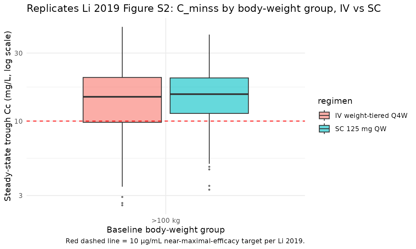

PKNCA validation

Non-compartmental analysis of the final (steady-state) SC and IV dosing intervals. Computes C_max, C_min, C_avg, and AUC per simulated subject and regimen.

nca_conc_sc <- sim_sc |>
  dplyr::filter(time >= ss_start_sc, time <= ss_end_sc, !is.na(Cc)) |>
  dplyr::mutate(time_nom = time - ss_start_sc) |>
  dplyr::select(id, time = time_nom, Cc, treatment)

nca_dose_sc <- cohort |>
  dplyr::mutate(time = 0, amt = 125, treatment = "SC_125_QW") |>
  dplyr::select(id, time, amt, treatment)

conc_obj_sc <- PKNCA::PKNCAconc(nca_conc_sc, Cc ~ time | treatment + id)
dose_obj_sc <- PKNCA::PKNCAdose(nca_dose_sc, amt ~ time | treatment + id)

intervals_sc <- data.frame(start = 0, end = tau_sc,
                           cmax = TRUE, cmin = TRUE, tmax = TRUE,
                           auclast = TRUE, cav = TRUE)
nca_sc <- PKNCA::pk.nca(PKNCA::PKNCAdata(conc_obj_sc, dose_obj_sc, intervals = intervals_sc))
#>  ■■■■■■■■■■■■■■■■■■■■■■■■          76% |  ETA:  1s
summary(nca_sc)
#>  start end treatment   N    auclast        cmax        cmin              tmax
#>      0   7 SC_125_QW 400 123 [38.1] 19.4 [35.7] 14.9 [44.0] 2.00 [1.00, 3.00]
#>          cav
#>  17.6 [38.1]
#> 
#> Caption: auclast, cmax, cmin, cav: geometric mean and geometric coefficient of variation; tmax: median and range; N: number of subjects

nca_conc_iv <- sim_iv |>
  dplyr::filter(time >= ss_start_iv, time <= ss_end_iv, !is.na(Cc)) |>
  dplyr::mutate(time_nom = time - ss_start_iv) |>
  dplyr::select(id, time = time_nom, Cc, treatment)

nca_dose_iv <- cohort_iv |>
  dplyr::mutate(time = 0, amt = amt_iv, treatment = "IV_weight_tiered_Q4W") |>
  dplyr::select(id, time, amt, treatment)

conc_obj_iv <- PKNCA::PKNCAconc(nca_conc_iv, Cc ~ time | treatment + id)
dose_obj_iv <- PKNCA::PKNCAdose(nca_dose_iv, amt ~ time | treatment + id)

intervals_iv <- data.frame(start = 0, end = tau_iv,
                           cmax = TRUE, cmin = TRUE, tmax = TRUE,
                           auclast = TRUE, cav = TRUE)
nca_iv <- PKNCA::pk.nca(PKNCA::PKNCAdata(conc_obj_iv, dose_obj_iv, intervals = intervals_iv))
#>  ■■■■■■■■■■■■■■■■■■■■              64% |  ETA:  1s
summary(nca_iv)
#>  start end            treatment   N     auclast       cmax        cmin
#>      0  28 IV_weight_tiered_Q4W 400 1340 [32.3] 224 [25.7] 14.2 [56.8]
#>                  tmax         cav
#>  0.000 [0.000, 0.000] 47.8 [32.3]
#> 
#> Caption: auclast, cmax, cmin, cav: geometric mean and geometric coefficient of variation; tmax: median and range; N: number of subjects

Comparison against the Li 2019 C_minss ≥10 μg/mL benchmark

Li 2019 reports that ~90% of patients achieved a steady-state trough concentration of at least 10 μg/mL on each of the approved regimens. The cohort-fraction check below is a direct numerical replicate of that claim.

pct_above <- trough_by_wtgrp |>
  dplyr::group_by(regimen, wt_group) |>
  dplyr::summarise(
    N              = dplyr::n(),
    pct_ge_10_mgL  = 100 * mean(Cc >= 10, na.rm = TRUE),
    median_Cmin    = median(Cc),
    .groups = "drop"
  )

knitr::kable(pct_above, digits = 1,
  caption = "Fraction of virtual subjects with steady-state trough Cc >= 10 mg/L by regimen and weight group (Li 2019: ~90% across all groups).")

Fraction of virtual subjects with steady-state trough Cc >= 10 mg/L by regimen and weight group (Li 2019: ~90% across all groups).
regimen	wt_group	N	pct_ge_10_mgL	median_Cmin
IV weight-tiered Q4W	>100 kg	400	74.5	14.8
SC 125 mg QW	>100 kg	400	84.5	15.4

Assumptions and deviations

Time-unit rescaling. Li 2019 reports CL, Q, and KA in per-hour units; the model file converts each to per-day by the factor of 24 to match the nlmixr2lib units$time = "day" convention. VC, VP, F, IIV variances, and residual-error magnitudes carry through unchanged.
MTX excluded from the final-model equation. Li 2019 Table 1B lists CL_MTX = -0.0405 (95% CI crosses zero, not significant at the 0.1% backward-elimination threshold) but the paper’s final-model covariate equation on p. 249 does not include the MTX term. This model implements the published final-model equation and therefore excludes MTX; the remaining 10 covariate effects from Table 1B are retained.
FORM_ABA_PHASE2 as model-specific covariate. The abatacept SC phase-2-vs-phase-3 formulation indicator is implemented inline in covariateData rather than registered as a canonical entry, per the nlmixr2lib policy that FORM_* covariates stay model-specific unless they clearly generalize across multiple drugs. The covariate is used only for the phase-2 trial SC data; set to 0 for all simulations of the approved commercial 125 mg SC QW regimen. checkModelConventions() flags this as a warning, which is an accepted exception.
Virtual-cohort covariate distributions. Li 2019 Table S3 (baseline demographics) is referenced in the paper but is not embedded in the PMC full text, so the virtual-cohort distributions are approximate: WT ~ N(70, 18) truncated to [40, 160]; AGE ~ N(50, 13) truncated to [18, 90]; ALB ~ N(4.0, 0.35) truncated to [2.5, 5.0] g/dL; CRCL ~ N(90, 25) truncated to [30, 180]; SWOL_28JOINT ~ rounded N(16, 6) truncated to [0, 28]; SEXF = 78% female; CONMED_NSAID = 55%. The reference values match the Li 2019 Methods narrative; the dispersions approximate a typical RA phase-3 cohort.
IV as instantaneous bolus. Li 2019 uses a zero-order infusion (the approved IV regimen is a 30-minute infusion). This simulation treats IV doses as an instantaneous bolus to central, which slightly overstates the early-post-dose Cmax but has no effect on AUC, trough, or half-life estimates. Users wanting exact infusion kinetics should set rate (or dur) in the rxode2 event table.
No subject-level observed data. Li 2019 does not release individual subject data; the figures reported here are a pure forward simulation of the published final-model parameters against a virtual cohort.

Errata

The published Li 2019 paper contains two items that a reviewer re-reading the source alongside this model should be aware of:

Albumin unit typo (Methods p. 248). Li 2019 Methods states “baseline albumin of 4.0 mg/dL” as a reference-subject covariate value. Normal adult serum albumin is ~4 g/dL; a value of 4 mg/dL is a factor of 1000 too low and is physiologically impossible. This is treated as a publication unit typo: the model codes the ALB reference as 4.0 g/dL, which is clinically sensible and matches other abatacept PK reports (e.g. the Orencia label). This unit is recorded in covariateData[[ALB]]$units as g/dL with an explicit note.
Table 1B caption vs final-model equation (Table 1 caption and Results p. 249). Table 1 is captioned “Parameter Estimates for (A) the Structural Part of Final PPK Model for Abatacept and (B) the Covariates of the Full PPK Model” — i.e. Table 1A is final but Table 1B is explicitly the full model. Table 1B’s 11th row (CL_MTX = -0.0405, 95% CI crossing zero) is not present in the published final-model covariate equation on p. 249. The operator decision for this extraction was to treat Table 1B’s 10 non-MTX estimates as the published final-model covariate values (matching the final-model equation exactly) and to drop CL_MTX; the paper does not separately tabulate post-backward-elimination covariate estimates. If Bristol-Myers Squibb ever publishes a separate table of final-model covariate estimates that differ from Table 1B, the values in this model should be refit against that source.