Tenofovir and tenofovir-diphosphate (Burns 2015) • nlmixr2lib

Model and source

Citation: Burns RN, Hendrix CW, Chaturvedula A. Population pharmacokinetics of tenofovir and tenofovir-diphosphate in healthy women. J Clin Pharmacol. 2015;55(6):629-638. doi:10.1002/jcph.461
Description: Two-compartment population PK model for plasma tenofovir after oral tenofovir disoproxil fumarate in healthy women, parameterised with micro-rate constants and first-order absorption with a lag time, linked by a first-order rate constant to a peripheral-blood-mononuclear-cell tenofovir-diphosphate compartment with first-order elimination; body weight on central volume, and a fixed adherence-adjustment bioavailability on self-administered (unobserved) doses.
Article: https://doi.org/10.1002/jcph.461 (PMC5008110, open access)
Supplement: Supplementary Table S1 (demographics) and Supplementary Figures S2-S6, available from the article’s landing page and from EuropePMC’s supplementaryFiles endpoint for PMC5008110.

Burns 2015 is the first tenofovir / tenofovir-diphosphate population PK model developed solely from healthy participants – the pre-exposure-prophylaxis target population – rather than from HIV-infected patients or a mixed cohort. That matters for the intracellular arm: the two earlier published models report tenofovir-diphosphate half-lives of 85.8 and 115.5 hours and plateau concentrations of 128-174 fmol per million cells, against this model’s 53.3 hours and a simulated steady-state trough of 49.9 fmol per million cells. The authors also use a linear tenofovir-to-tenofovir-diphosphate link rather than the saturable one used by their predecessors, on the grounds that MTN-001 studied only the single clinically relevant 300 mg dose and so could not interrogate saturation.

Population

MTN-001 was a 21-week Phase II open-label three-period crossover study in which healthy, HIV-negative, non-pregnant women aged 18-45 received daily oral tenofovir disoproxil fumarate 300 mg (oral period), 1% vaginal tenofovir gel (vaginal period), or both (dual period), each for six weeks and separated by one-week washouts. 168 women enrolled and 144 completed at least one follow-up visit in each period.

Only the oral period’s end-of-period visit contributed to model building; the dual period was held back for internal qualification and the vaginal-only period was not modelled. Of 141 participants with PK measurements, 101 entered the analysis, contributing 476 plasma tenofovir and 399 PBMC tenofovir-diphosphate concentrations. Supplementary Table S1 reports the analysis cohort as mean (range): age 31.3 (18-45) years, weight 79.6 (43-145) kg, creatinine clearance 130.1 (64-257) mL/min, with 32 White, 60 Black and 9 Other participants. The weight median of 73 kg – the value used to centre the weight covariate – comes from the Results text rather than Table S1.

The same information is available programmatically from the model’s population metadata:

pop <- rxode2::rxode(readModelDb("Burns_2015_tenofovir"))$population
#> ℹ parameter labels from comments will be replaced by 'label()'
str(pop, max.level = 1)
#> List of 16
#>  $ species       : chr "human"
#>  $ n_subjects    : num 101
#>  $ n_observations: num 875
#>  $ n_studies     : num 1
#>  $ age_range     : chr "18-45 years"
#>  $ age_mean      : chr "31.3 years"
#>  $ weight_range  : chr "43-145 kg"
#>  $ weight_mean   : chr "79.6 kg"
#>  $ weight_median : chr "73 kg"
#>  $ sex_female_pct: num 100
#>  $ race_ethnicity: Named num [1:3] 32 60 9
#>   ..- attr(*, "names")= chr [1:3] "White" "Black" "Other"
#>  $ disease_state : chr "healthy HIV-negative women (pre-exposure prophylaxis target population)"
#>  $ renal_function: chr "creatinine clearance mean 130.1 (range 64-257) mL/min"
#>  $ dose_range    : chr "tenofovir disoproxil fumarate 300 mg orally once daily (136 mg tenofovir equivalents = 472.058 umol)"
#>  $ regions       : chr "United States, South Africa, Uganda, Zimbabwe (MTN-001 sites)"
#>  $ notes         : chr "MTN-001, a 21-week Phase II open-label three-period crossover study of daily oral tenofovir disoproxil fumarate"| __truncated__

Source trace

The per-parameter origin is recorded as an in-file comment next to each ini() entry in inst/modeldb/specificDrugs/Burns_2015_tenofovir.R. The table below collects them in one place. All values are the Final Model column of Table 1; the Base Model column (no weight covariate) is not extracted.

Equation / parameter	Value	Source location
`lka` (KA)	9.79 1/h	Table 1, final model, “KA (h-1)” (65.18% RSE)
`lvc` (Vc/F at 73 kg)	385.71 L	Table 1, final model, “Vc/F (L)” (14.84% RSE)
`e_wt_vc` (weight on Vc)	-2.16 L/kg	Table 1, final model, “cov WT (kg) on Vc” (34.52% RSE); bootstrap median -1.78, 95% CI -3.37 to -0.16
`lk12` (K23)	0.631 1/h	Table 1, final model, “K23 (h-1)” (24.7% RSE)
`lk21` (K32)	0.396 1/h	Table 1, final model, “K32 (h-1)” (23.24% RSE)
`lkel` (K20)	0.13 1/h	Table 1, final model, “K20 (h-1)” (17.81% RSE)
`lkmet_tfvdp` (K24)	0.017 1/h	Table 1, final model, “K24 (h-1)” (72.48% RSE)
`lkel_tfvdp` (K40)	0.013 1/h	Table 1, final model, “K40 (h-1)” (16.63% RSE)
`ltlag` (absorption lag)	0.5 h	Table 1, final model, “Absorption lag (h)” (35.49% RSE)
`lfdepot` (F1, fixed)	0.5	Methods, “Nonadherence…”: F1 fixed to 0.5; Table 1 footnote confirms the F1 row holds empirical Bayes estimates, not an estimated typical value
`etalfdepot` (fixed)	variance 10	Methods, “…and its omega distribution to a high value, in our case 10”
`etalka`	160.16% CV	Results text (Table 1 rounds to 160.2); converted as `log(1 + CV^2)`
`etalvc`	19.3% CV	Table 1, final model, “BSV Vc (%CV)”
`etalkel`	36.22% CV	Table 1, final model, “BSV K20 (%CV)”
`etalkmet_tfvdp`	159.49% CV	Table 1, final model, “BSV K24 (%CV)”
`propSd`	27.48% CV	Table 1, final model, “Proportional, TFV (%CV)”
`propSd_Cpbmc_tfvdp`	31.18% CV	Table 1, final model, “Proportional, TFV-DP (PBMC) (%CV)”
Structural model (4 states, micro-rate constants)	n/a	Supplementary Figure S2 (“Structural model overview”); Methods, “TFV and TFV-DP were modeled simultaneously…”
Weight covariate equation	n/a	Results: “TVV = 385.71 - 2.16 * (73 - weight (kg))”
Between-subject variability form	n/a	Methods: “theta_i = theta_typical * exp(eta_i)”
Adherence bioavailability form	n/a	Methods: “F1 = 0.5 * exp(eta_i)” (Gibiansky’s method)
Molar dose conversion	472.058 umol	Methods: “136 mg TFV/300 mg TDF … in micromoles … (TFV molecular weight of 288.1 g/mole)”
PBMC volume conversion	282 fL/cell	Methods: “converted to nanomoles/L using a PBMC cell volume of 282 femtoliters/cell”

Units and the two unit conversions

Two conversions are load-bearing and are set up once here.

# One 300 mg tenofovir disoproxil fumarate tablet = 136 mg tenofovir
# equivalents; tenofovir molecular weight 288.1 g/mol (Methods).
MW_TFV <- 288.1
DOSE_UMOL <- 136 / MW_TFV * 1000
DOSE_UMOL
#> [1] 472.0583

# Tenofovir-diphosphate was assayed as fmol per million PBMC and converted to
# nmol/L for modelling, using a PBMC volume of 282 fL/cell (Methods). One
# fmol per million cells is therefore this many nmol/L:
FMOL_TO_NM <- 1e-6 / (282e-15 * 1e6)
FMOL_TO_NM
#> [1] 3.546099

The plasma tenofovir observation Cc is central / vc, i.e. umol / L = nmol/mL, exactly as drawn in Supplementary Figure S2 (“Plasma, TFV nm/ml”).

The tenofovir-diphosphate observation Cpbmc_tfvdp is the compartment content read directly, with no volume term. The authors fitted in NONMEM ADVAN5, no scaling parameter for compartment 4 is reported anywhere in the paper, and Figure S2 labels the PBMC box “PBMC, TFV-DP nm/L” with no volume – so the NONMEM default scale of 1 applies and the whole amount-to-concentration conversion is absorbed into the apparent K24. The Discussion says as much: “we modeled only 1 million PBMCs and thus the parameters were apparent in theory”. The section “Steady-state tenofovir-diphosphate” below checks that reading against a number the model was not fitted to.

Structural identities

Three quantities quoted in the paper are exact algebraic consequences of the tabulated micro-rate constants. They are deterministic – no simulation, no random draws – so they are asserted tightly.

ui <- rxode2::rxode(readModelDb("Burns_2015_tenofovir"))
#> ℹ parameter labels from comments will be replaced by 'label()'
th <- ui$theta

ka  <- exp(th[["lka"]])
vc  <- exp(th[["lvc"]])
kel <- exp(th[["lkel"]])
k12 <- exp(th[["lk12"]])
k21 <- exp(th[["lk21"]])
kmet <- exp(th[["lkmet_tfvdp"]])
kel_dp <- exp(th[["lkel_tfvdp"]])

# 1. Total apparent tenofovir clearance. Results is explicit that K24 is a
#    second apparent clearance route and must be included: "if TFV
#    micro-constants K20 and K24 are converted to clearance terms
#    ((K24 + K20)*Vc), our model yields a mean total apparent clearance of ...
#    56.7 L/h for the final model".
cl_apparent <- (kel + kmet) * vc

# 2. Tenofovir-diphosphate half-life: "The population estimate for elimination
#    of TFV-DP in the final model was 0.013 h-1 which yields a half-life of
#    53.3 hours" (Results).
t_half_dp <- log(2) / kel_dp

# 3. Vc/F at the extremes of the observed weight range (43-145 kg,
#    Supplementary Table S1) under the published linear equation.
vc_at <- function(wt) vc + th[["e_wt_vc"]] * (73 - wt)

identities <- tibble::tibble(
  Quantity = c(
    "Total apparent CL/F = (K20 + K24) * Vc (L/h)",
    "TFV-DP half-life = log(2) / K40 (h)",
    "Molar dose per 300 mg TDF tablet (umol)",
    "Vc/F at 43 kg (L)",
    "Vc/F at 73 kg, the centring weight (L)",
    "Vc/F at 145 kg (L)"
  ),
  Model = c(cl_apparent, t_half_dp, DOSE_UMOL, vc_at(43), vc_at(73), vc_at(145)),
  Published = c(56.7, 53.3, NA, NA, 385.71, NA)
) |>
  dplyr::mutate(`% diff` = 100 * (Model - Published) / Published)

knitr::kable(identities, digits = 2,
             caption = "Closed-form identities against values quoted in Burns 2015.")

Closed-form identities against values quoted in Burns 2015.
Quantity	Model	Published	% diff
Total apparent CL/F = (K20 + K24) * Vc (L/h)	56.70	56.70	0.00
TFV-DP half-life = log(2) / K40 (h)	53.32	53.30	0.04
Molar dose per 300 mg TDF tablet (umol)	472.06	NA	NA
Vc/F at 43 kg (L)	320.91	NA	NA
Vc/F at 73 kg, the centring weight (L)	385.71	385.71	0.00
Vc/F at 145 kg (L)	541.23	NA	NA


stopifnot(
  # Both published quantities are exact functions of the tabulated estimates,
  # so the only tolerance needed is the paper's own rounding to 3 significant
  # figures. Achieved: 56.70 vs 56.7 and 53.32 vs 53.3.
  abs(cl_apparent - 56.7) < 0.1,
  abs(t_half_dp - 53.3) < 0.1,
  # Vc/F must rise with weight under the published equation -- this is the one
  # place a sign slip in a linear centred covariate would hide, because both
  # signs give physically plausible volumes across 43-145 kg.
  vc_at(43) < vc_at(73), vc_at(73) < vc_at(145),
  abs(vc_at(73) - 385.71) < 0.01
)

Single-dose profile and PKNCA

The paper’s external qualification simulated a single 300 mg tenofovir disoproxil fumarate dose (Louissaint 2013, six healthy premenopausal women, 15 days of sampling) and compared the prediction interval against the observed data. We reproduce that design at typical values so the NCA below is deterministic, then run PKNCA on both analytes.

Doses are given with SELFADMIN = 0 throughout: every simulation in this vignette assumes full compliance with observed dosing, which is what the authors assumed for their qualification runs. The adherence bioavailability is exercised separately in the last section.

mod <- readModelDb("Burns_2015_tenofovir")
mod_typical <- rxode2::zeroRe(mod)
#> ℹ parameter labels from comments will be replaced by 'label()'

# Dense early grid to resolve Tmax (absorption is fast: KA = 9.79 1/h behind a
# 0.5 h lag), then coarser out to 15 days to capture the tenofovir-diphosphate
# terminal phase.
grid_sd <- sort(unique(c(
  seq(0, 12, by = 0.05),
  seq(12, 24, by = 0.25),
  seq(24, 360, by = 2)
)))

events_sd <- dplyr::bind_rows(
  data.frame(id = 1L, time = 0, amt = DOSE_UMOL, evid = 1L,
             cmt = "depot", dvid = NA_integer_),
  data.frame(id = 1L, time = grid_sd, amt = NA_real_, evid = 0L,
             cmt = "central", dvid = 1L)
) |>
  dplyr::mutate(WT = 73, SELFADMIN = 0) |>
  dplyr::arrange(id, time, dplyr::desc(evid))

# useLinCmt = FALSE: rxode2's automatic ODE -> linCmt conversion corrupts the
# dvid -> cmt mapping for multi-output models.
sim_sd <- rxode2::rxSolve(mod_typical, events_sd, returnType = "data.frame",
                          useLinCmt = FALSE)
#> ℹ omega/sigma items treated as zero: 'etalka', 'etalvc', 'etalkel', 'etalkmet_tfvdp', 'etalfdepot'

# Both algebraic observables come back as columns on every observation row,
# regardless of which dvid the row carries.
stopifnot(all(c("Cc", "Cpbmc_tfvdp") %in% names(sim_sd)),
          nrow(sim_sd) > 0,
          all(sim_sd$Cc >= 0), all(sim_sd$Cpbmc_tfvdp >= 0))

# Replicates the shape of Figure 4 of Burns 2015 (single-dose external
# qualification): plasma tenofovir and PBMC tenofovir-diphosphate after one
# 300 mg TDF dose. The published figure overlays six individuals' observed
# data, which are not redistributable here, so only the typical-value
# prediction is drawn.
sim_sd |>
  dplyr::transmute(
    time,
    `Plasma tenofovir (ng/mL)` = Cc * MW_TFV,
    `PBMC tenofovir-diphosphate (fmol per 1e6 cells)` = Cpbmc_tfvdp / FMOL_TO_NM
  ) |>
  tidyr::pivot_longer(-time, names_to = "analyte", values_to = "value") |>
  dplyr::filter(value > 0) |>
  ggplot(aes(time / 24, value)) +
  geom_line() +
  facet_wrap(~analyte, scales = "free_y") +
  scale_y_log10() +
  labs(x = "Time (days)", y = NULL,
       title = "Single 300 mg TDF dose, typical values",
       caption = "Replicates the design of Figure 4 of Burns 2015.")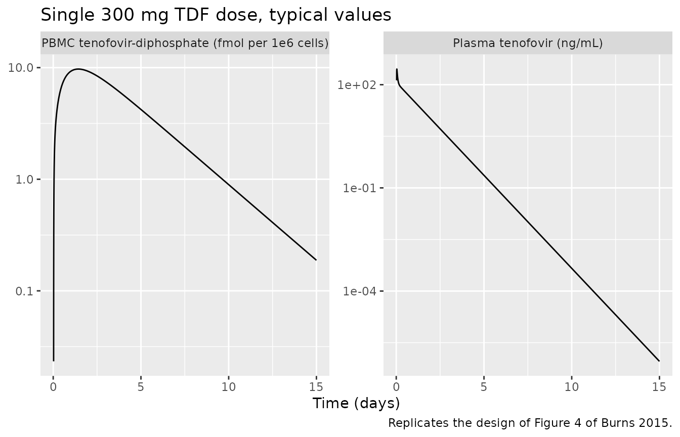

# PKNCA input: filter on !is.na() ONLY. Adding time > 0 or Cc > 0 would drop
# the time-zero row that anchors AUC0-inf.
nca_conc <- sim_sd |>
  dplyr::filter(!is.na(Cc)) |>
  dplyr::mutate(id = 1L, treatment = "TDF 300 mg single dose") |>
  dplyr::select(id, treatment, time, Cc, Cpbmc_tfvdp)

# Guarantee a time-zero record per (id, treatment); pre-dose extravascular
# concentration is 0 for both analytes.
nca_conc <- dplyr::bind_rows(
  nca_conc,
  nca_conc |> dplyr::distinct(id, treatment) |>
    dplyr::mutate(time = 0, Cc = 0, Cpbmc_tfvdp = 0)
) |>
  dplyr::distinct(id, treatment, time, .keep_all = TRUE) |>
  dplyr::arrange(id, treatment, time)

dose_obj <- PKNCA::PKNCAdose(
  data.frame(id = 1L, treatment = "TDF 300 mg single dose",
             time = 0, amt = DOSE_UMOL),
  amt ~ time | treatment + id
)

# One PKNCA block per output (multi-output model).
res_tfv <- PKNCA::pk.nca(PKNCA::PKNCAdata(
  PKNCA::PKNCAconc(nca_conc, Cc ~ time | treatment + id),
  dose_obj,
  intervals = data.frame(start = 0, end = Inf, cmax = TRUE, tmax = TRUE,
                         aucinf.obs = TRUE, half.life = TRUE, cl.obs = TRUE)
))

res_dp <- PKNCA::pk.nca(PKNCA::PKNCAdata(
  PKNCA::PKNCAconc(nca_conc, Cpbmc_tfvdp ~ time | treatment + id),
  dose_obj,
  intervals = data.frame(start = 0, end = Inf, cmax = TRUE, tmax = TRUE,
                         aucinf.obs = TRUE, half.life = TRUE)
))

pick <- function(res, code) {
  v <- as.data.frame(res)$PPORRES[as.data.frame(res)$PPTESTCD == code]
  if (length(v) != 1L) stop("no unique PKNCA row for '", code, "'")
  v
}

nca_summary <- tibble::tibble(
  Analyte = c(rep("Plasma tenofovir", 4L),
              rep("PBMC tenofovir-diphosphate", 4L)),
  Parameter = rep(c("Cmax", "Tmax (h)", "AUC0-inf", "Half-life (h)"), 2L),
  Value = c(
    pick(res_tfv, "cmax") * MW_TFV, pick(res_tfv, "tmax"),
    pick(res_tfv, "aucinf.obs") * MW_TFV, pick(res_tfv, "half.life"),
    pick(res_dp, "cmax") / FMOL_TO_NM, pick(res_dp, "tmax"),
    pick(res_dp, "aucinf.obs") / FMOL_TO_NM, pick(res_dp, "half.life")
  ),
  Units = c("ng/mL", "h", "ng*h/mL", "h",
            "fmol per 1e6 cells", "h", "fmol*h per 1e6 cells", "h")
)

knitr::kable(nca_summary, digits = 2,
             caption = paste("PKNCA on the typical-value single-dose profile.",
                             "Cmax / AUC converted from the model's molar",
                             "scale into the paper's display units."))

PKNCA on the typical-value single-dose profile. Cmax / AUC converted from the model’s molar scale into the paper’s display units.
Analyte	Parameter	Value	Units
Plasma tenofovir	Cmax	284.81	ng/mL
Plasma tenofovir	Tmax (h)	0.80	h
Plasma tenofovir	AUC0-inf	2397.88	ng*h/mL
Plasma tenofovir	Half-life (h)	13.33	h
PBMC tenofovir-diphosphate	Cmax	9.71	fmol per 1e6 cells
PBMC tenofovir-diphosphate	Tmax (h)	34.00	h
PBMC tenofovir-diphosphate	AUC0-inf	1184.27	fmol*h per 1e6 cells
PBMC tenofovir-diphosphate	Half-life (h)	53.76	h

Comparison against published NCA

Burns 2015 does not tabulate an NCA of its own, but it quotes two quantities that NCA on a simulated single-dose profile recovers directly: the total apparent tenofovir clearance and the tenofovir-diphosphate half-life. Both are independent checks that the micro-rate-constant parameterisation, the molar dose conversion and the unscaled tenofovir-diphosphate compartment were all transcribed consistently – a mis-set volume or dose unit moves cl.obs by the same factor it moves the dose.

simulated_wide <- tibble::tibble(
  analyte = c("Plasma tenofovir", "PBMC tenofovir-diphosphate"),
  cl.obs = c(pick(res_tfv, "cl.obs"), NA_real_),
  half.life = c(pick(res_tfv, "half.life"), pick(res_dp, "half.life"))
)

published_wide <- tibble::tibble(
  analyte = c("Plasma tenofovir", "PBMC tenofovir-diphosphate"),
  # Abstract and Discussion: "apparent TFV clearance of 56.7 L/h
  # ((K20 + K24)*Vc)".
  cl.obs = c(56.7, NA_real_),
  # Results: TFV-DP "half-life was 53.3 hours". Tenofovir's own terminal
  # half-life is not reported by the paper, so it is left blank rather than
  # compared against a number from elsewhere.
  half.life = c(NA_real_, 53.3)
)

cmp <- nlmixr2lib::ncaComparisonTable(
  simulated = simulated_wide,
  reference = published_wide,
  by = "analyte",
  units = c(cl.obs = "L/h", half.life = "h"),
  tolerance_pct = 20,
  label_first_column = "NCA parameter"
)

knitr::kable(
  cmp,
  caption = "Simulated vs. published values. * differs from reference by >20%."
)

Simulated vs. published values. * differs from reference by >20%.
NCA parameter	analyte	Reference	Simulated	% diff
t½ (h)	Plasma tenofovir	—	13.3	—
t½ (h)	PBMC tenofovir-diphosphate	53.3	53.8	+0.9%
CL/F (L/h)	Plasma tenofovir	56.7	56.7	+0.0%
CL/F (L/h)	PBMC tenofovir-diphosphate	—	—	—


stopifnot(
  # Deterministic (typical-value) quantities, so these are tight. Achieved
  # 56.72 vs 56.7 (0.03%) and 53.8 vs 53.3 (0.9%; the small positive bias is
  # the NCA terminal-slope window, not the model -- log(2)/K40 is exact, and
  # asserted to 0.1 h in the identities section above).
  abs(100 * (pick(res_tfv, "cl.obs") - 56.7) / 56.7) < 1,
  abs(100 * (pick(res_dp, "half.life") - 53.3) / 53.3) < 3
)

The tenofovir-diphosphate terminal phase is elimination-rate-limited rather than formation-limited, which is what makes its NCA half-life recover K40: the paper constrained K24 (0.017 1/h) to exceed K40 (0.013 1/h) for exactly this reason, and tenofovir’s own terminal half-life is 13.3 hours – four times faster than the intracellular pool it feeds.

Steady-state tenofovir-diphosphate

This is the paper’s most informative qualification result and the one that is not circular: the authors simulated 16 daily 300 mg doses at the median weight of 73 kg, assuming full compliance, and compared the resulting tenofovir-diphosphate trough against the directly-observed-therapy STRAND trial, which the model was never fitted to. They report a simulated median trough of 49.9 fmol per million cells (IQR 34.1-74.7) against STRAND’s observed median of 42 (IQR 31-47).

It is also the check that settles how the tenofovir-diphosphate compartment is scaled. Reading the compartment content directly as nmol/L – the NONMEM default of 1 – lands on the published trough. Introducing any genuine PBMC volume in its place (2.82e-7 L for a million cells) would miss it by roughly nine orders of magnitude.

# set.seed() seeds R's RNG. It does NOT seed rxode2's simulation RNG, whose
# streams are partitioned per solver thread -- so this cohort differs between a
# 2-core CI runner and a 16-thread workstation, and no seed makes them agree.
# Every assertion below is therefore written on a centre or a robust quantile,
# never on an extreme.
set.seed(20150601)

N_SUB <- 200L

# Weight: Supplementary Table S1 reports mean 79.6 kg and range 43-145 kg, and
# Results gives the median as 73 kg. Mean > median means the distribution is
# right-skewed, so a log-normal centred on the median and truncated to the
# reported range is assumed (see Assumptions).
draw_weight <- function(n) {
  wt <- numeric(0)
  while (length(wt) < n) {
    cand <- stats::rlnorm(2 * n, meanlog = log(73), sdlog = 0.416)
    wt <- c(wt, cand[cand >= 43 & cand <= 145])
  }
  wt[seq_len(n)]
}

cohort <- tibble::tibble(id = seq_len(N_SUB), WT = draw_weight(N_SUB))

# 16 daily doses, as the paper simulated. The last dose is at 360 h and none
# follows, so t = 384 h is the 16th interval's trough.
#
# Coarse grid over the accumulation phase (the tenofovir-diphosphate pool has a
# 53 h half-life and moves slowly), then a fine grid over the final interval so
# that plasma Tmax is resolved -- absorption is fast (KA = 9.79 1/h behind a
# 0.5 h lag), and a coarse grid there would understate Cmax badly. The two
# ranges are disjoint so no de-duplication is needed.
dose_times <- seq(0, by = 24, length.out = 16L)
obs_times <- c(seq(0, 354, by = 6), seq(360, 384, by = 0.5))

events_ss <- dplyr::bind_rows(
  tidyr::crossing(cohort, time = dose_times) |>
    dplyr::mutate(amt = DOSE_UMOL, evid = 1L, cmt = "depot",
                  dvid = NA_integer_),
  tidyr::crossing(cohort, time = obs_times) |>
    dplyr::mutate(amt = NA_real_, evid = 0L, cmt = "central", dvid = 1L)
) |>
  dplyr::mutate(SELFADMIN = 0) |>
  dplyr::arrange(id, time, dplyr::desc(evid))

stopifnot(!anyDuplicated(unique(events_ss[, c("id", "time", "evid")])))

sim_ss <- rxode2::rxSolve(mod, events_ss, returnType = "data.frame",
                          keep = c("WT"), useLinCmt = FALSE)
#> ℹ parameter labels from comments will be replaced by 'label()'

sim_ss <- sim_ss |>
  dplyr::mutate(tfvdp_fmol = Cpbmc_tfvdp / FMOL_TO_NM)

# Replicates Figure 5 of Burns 2015: multiple-dose simulation to steady state,
# median and 90% prediction interval of PBMC tenofovir-diphosphate.
sim_ss |>
  dplyr::group_by(time) |>
  dplyr::summarise(
    Q05 = quantile(tfvdp_fmol, 0.05),
    Q50 = quantile(tfvdp_fmol, 0.50),
    Q95 = quantile(tfvdp_fmol, 0.95),
    .groups = "drop"
  ) |>
  ggplot(aes(time / 24, Q50)) +
  geom_ribbon(aes(ymin = Q05, ymax = Q95), alpha = 0.25) +
  geom_line() +
  geom_hline(yintercept = 49.9, linetype = "dashed", colour = "firebrick") +
  labs(x = "Time (days)", y = "PBMC TFV-DP (fmol per 1e6 cells)",
       title = "16 daily 300 mg TDF doses, full compliance",
       caption = paste("Replicates Figure 5 of Burns 2015. Dashed line:",
                       "the paper's simulated steady-state median trough",
                       "of 49.9 fmol per million cells."))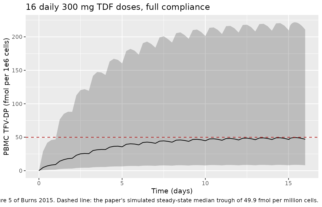

# The paper read its trough "after 265 hours, ~5 TFV-DP half-lives"; the last
# dosing interval of the 16-dose regimen ends at 384 h.
trough_time <- max(dose_times) + 24

cohort_trough <- sim_ss |>
  dplyr::filter(time == trough_time) |>
  dplyr::pull(tfvdp_fmol)
stopifnot(length(cohort_trough) == N_SUB)

# Typical-value (zeroRe) counterpart at the paper's stated 73 kg.
events_ss_typ <- events_ss |>
  dplyr::filter(id == 1L) |>
  dplyr::mutate(WT = 73)
typical_trough <- rxode2::rxSolve(
  mod_typical, events_ss_typ, returnType = "data.frame", useLinCmt = FALSE
) |>
  dplyr::filter(time == trough_time) |>
  dplyr::pull(Cpbmc_tfvdp) / FMOL_TO_NM
#> ℹ omega/sigma items treated as zero: 'etalka', 'etalvc', 'etalkel', 'etalkmet_tfvdp', 'etalfdepot'
stopifnot(length(typical_trough) == 1L)

trough_tab <- tibble::tibble(
  Statistic = c("Typical value (73 kg, no IIV)",
                "Cohort median", "Cohort 1st quartile", "Cohort 3rd quartile"),
  Model = c(typical_trough, quantile(cohort_trough, c(0.5, 0.25, 0.75))),
  `Burns 2015 simulation` = c(NA, 49.9, 34.1, 74.7),
  `STRAND observed` = c(NA, 42, 31, 47)
)

knitr::kable(trough_tab, digits = 1,
             caption = paste("Steady-state PBMC tenofovir-diphosphate trough,",
                             "fmol per million cells."))

Steady-state PBMC tenofovir-diphosphate trough, fmol per million cells.
Statistic	Model	Burns 2015 simulation	STRAND observed
Typical value (73 kg, no IIV)	47.1	NA	NA
Cohort median	46.8	49.9	42
Cohort 1st quartile	24.2	34.1	31
Cohort 3rd quartile	96.2	74.7	47


pct_typical <- 100 * (typical_trough - 49.9) / 49.9
pct_median <- 100 * (median(cohort_trough) - 49.9) / 49.9

stopifnot(
  # Typical-value trough: deterministic, so a tight bound. Achieved -5.5%
  # (47.1 against 49.9). The residual gap is that the paper's 49.9 is a MEDIAN
  # OVER A SIMULATED COHORT, and the steady-state trough is a saturating
  # function of K24 (proportional to K24 / (K20 + K24)), so a cohort median
  # need not coincide with the typical-value prediction.
  abs(pct_typical) < 10,
  # Cohort median: robust to which subjects land in the tails, but still a
  # simulated quantity, so the bound has real headroom over the observed
  # spread. Realised -6.1% at every one of 1, 2, 4 and 16 solver threads while
  # authoring; 20 still breaks on a mis-transcribed K24, K40, dose or volume,
  # each of which moves the trough by tens of percent or more.
  abs(pct_median) < 20,
  # The pool must actually have accumulated: a trough at 16 days has to be
  # many-fold above the single-dose Cmax of the same pool.
  median(cohort_trough) > 3 * pick(res_dp, "cmax") / FMOL_TO_NM
)

Known deviation: the simulated interquartile range is wider than the paper’s. This cohort reproduces the paper’s median well but spreads roughly twice as far (IQR about 24-96 against the published 34.1-74.7). The cause is identified and is not a transcription error: Burns 2015 states that the inflated variance on the adherence bioavailability made ordinary Monte-Carlo simulation produce “exaggerated prediction intervals”, and that they therefore imputed individual empirical Bayes estimates instead of sampling. Empirical Bayes estimates are shrunk toward the population mean – heavily so for K24, whose 159% CV was estimated from sparse data at 72% RSE – so any EBE-based simulation is narrower than one that samples the full published omega. Sampling the published omega, as here, is the faithful reading of the model file; the paper’s narrower interval is a property of its simulation procedure, not of its parameter estimates. The gate above is therefore placed on the median and not on the quartiles.

Steady-state plasma tenofovir

# Replicates the shape of Figure 2 of Burns 2015 (final-model VPC over one
# dosing interval): plasma tenofovir, median and 90% prediction interval.
sim_ss |>
  dplyr::filter(time >= 360, time <= 384) |>
  dplyr::mutate(tad = time - 360) |>
  dplyr::group_by(tad) |>
  dplyr::summarise(
    Q05 = quantile(Cc * MW_TFV, 0.05),
    Q50 = quantile(Cc * MW_TFV, 0.50),
    Q95 = quantile(Cc * MW_TFV, 0.95),
    .groups = "drop"
  ) |>
  ggplot(aes(tad, Q50)) +
  geom_ribbon(aes(ymin = Q05, ymax = Q95), alpha = 0.25) +
  geom_line() +
  labs(x = "Time after dose (h)", y = "Plasma tenofovir (ng/mL)",
       title = "Plasma tenofovir over the 16th dosing interval",
       caption = "Replicates the layout of Figure 2 of Burns 2015.")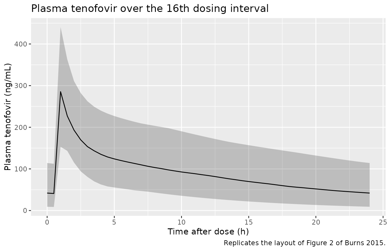

# Burns 2015 reports no plasma NCA, so this is a range check against the
# tenofovir literature the paper itself appeals to ("Our parameter estimates
# for TFV were in agreement with literature values"), not a published-value
# gate: steady-state 300 mg TDF gives Cmax of order 300 ng/mL and a trough of
# order 50 ng/mL.
tfv_ss <- sim_ss |>
  dplyr::filter(time >= 360, time <= 384) |>
  dplyr::group_by(id) |>
  dplyr::summarise(cmax = max(Cc) * MW_TFV,
                   ctrough = dplyr::last(Cc[order(time)]) * MW_TFV,
                   .groups = "drop")

knitr::kable(
  tibble::tibble(
    Statistic = c("Cmax (ng/mL)", "Ctrough (ng/mL)"),
    Median = c(median(tfv_ss$cmax), median(tfv_ss$ctrough)),
    `5th pct` = c(quantile(tfv_ss$cmax, 0.05), quantile(tfv_ss$ctrough, 0.05)),
    `95th pct` = c(quantile(tfv_ss$cmax, 0.95), quantile(tfv_ss$ctrough, 0.95))
  ),
  digits = 1,
  caption = "Simulated steady-state plasma tenofovir over the 16th interval."
)

Simulated steady-state plasma tenofovir over the 16th interval.
Statistic	Median	5th pct	95th pct
Cmax (ng/mL)	286.4	164.4	440.6
Ctrough (ng/mL)	42.0	9.1	114.1


stopifnot(
  # Broad order-of-magnitude bounds on the cohort MEDIAN, wide enough to be
  # insensitive to which cohort is drawn but narrow enough that a wrong molar
  # dose (a factor of 2.2 if the 300 mg TDF mass were used in place of the
  # 136 mg tenofovir-equivalent mass) or a wrong volume breaks them.
  median(tfv_ss$cmax) > 150, median(tfv_ss$cmax) < 600,
  median(tfv_ss$ctrough) > 20, median(tfv_ss$ctrough) < 120
)

Weight covariate

# Deterministic sweep across the observed weight range, at steady state.
wt_grid <- c(43, 60, 73, 100, 145)

events_wt <- dplyr::bind_rows(
  tidyr::crossing(tibble::tibble(id = seq_along(wt_grid), WT = wt_grid),
                  time = dose_times) |>
    dplyr::mutate(amt = DOSE_UMOL, evid = 1L, cmt = "depot",
                  dvid = NA_integer_),
  tidyr::crossing(tibble::tibble(id = seq_along(wt_grid), WT = wt_grid),
                  time = seq(360, 384, by = 0.25)) |>
    dplyr::mutate(amt = NA_real_, evid = 0L, cmt = "central", dvid = 1L)
) |>
  dplyr::mutate(SELFADMIN = 0) |>
  dplyr::arrange(id, time, dplyr::desc(evid))

sim_wt <- rxode2::rxSolve(mod_typical, events_wt, returnType = "data.frame",
                          keep = c("WT"), useLinCmt = FALSE)
#> ℹ omega/sigma items treated as zero: 'etalka', 'etalvc', 'etalkel', 'etalkmet_tfvdp', 'etalfdepot'
#> Warning: multi-subject simulation without without 'omega'

wt_tab <- sim_wt |>
  dplyr::filter(time >= 360) |>
  dplyr::group_by(WT) |>
  dplyr::summarise(
    `Vc/F (L)` = mean(vc),
    `TFV Cmax (ng/mL)` = max(Cc) * MW_TFV,
    `TFV-DP trough (fmol per 1e6 cells)` =
      dplyr::last(Cpbmc_tfvdp[order(time)]) / FMOL_TO_NM,
    .groups = "drop"
  ) |>
  dplyr::rename("Weight (kg)" = WT)

knitr::kable(wt_tab, digits = 2,
             caption = paste("Typical-value steady-state exposure across the",
                             "observed weight range (43-145 kg)."))

Typical-value steady-state exposure across the observed weight range (43-145 kg).
Weight (kg)	Vc/F (L)	TFV Cmax (ng/mL)	TFV-DP trough (fmol per 1e6 cells)
43	320.91	395.27	47.15
60	357.63	354.69	47.15
73	385.71	328.87	47.15
100	444.03	285.67	47.15
145	541.23	234.37	47.15


stopifnot(
  # The covariate acts on volume only, so it must move Cmax and leave the
  # tenofovir-diphosphate trough essentially untouched: the intracellular
  # pool is driven by the central AMOUNT through K24, which no volume term
  # enters. This is a structural consequence, not a fitted result, so it is
  # asserted tightly on deterministic values.
  wt_tab$`TFV Cmax (ng/mL)`[wt_tab$`Weight (kg)` == 43] >
    wt_tab$`TFV Cmax (ng/mL)`[wt_tab$`Weight (kg)` == 145],
  diff(range(wt_tab$`TFV-DP trough (fmol per 1e6 cells)`)) < 1e-6
)

Weight enters the central volume only, so it shifts plasma tenofovir concentrations (a 145 kg woman has about 69% higher Vc/F than a 43 kg woman and correspondingly lower peak concentrations) while leaving intracellular tenofovir-diphosphate exactly unchanged. That is a structural property of this model, not an empirical finding: the tenofovir-diphosphate compartment is fed by K24 * central, an amount, into which no volume enters.

The adherence adjustment

The methodological contribution of Burns 2015 is its handling of suspected non-adherence in MTN-001. Following Gibiansky’s method, the self-reported dose taken at home the day before the clinic visit carries a bioavailability fixed at 0.5 with a deliberately enormous fixed between-subject variance (10 on the log scale), while the observed in-clinic dose has bioavailability 1. The wide prior is close to uninformative, so each subject’s empirical Bayes estimate is driven by their own pre-dose concentration and can absorb either a missed dose or an extra one – the reported estimates ranged from 0.015 to 4.17 with a mean of 0.98.

In this model file that split is carried by the canonical SELFADMIN column: SELFADMIN = 1 marks the unobserved home dose, SELFADMIN = 0 the observed one. Set SELFADMIN = 0 on every dose to simulate full compliance, which is what every section above does and what the paper assumed for its qualification runs.

# Reproduce the estimation dataset's dosing structure for one subject: an
# unobserved dose 12 h before an observed in-clinic dose (Methods: the
# preclinic dose was a mean of 12.9 h, range 1.95-35 h, before the clinic
# dose).
adherence_case <- function(selfadmin_f1) {
  dplyr::bind_rows(
    data.frame(id = 1L, time = 0, amt = DOSE_UMOL, evid = 1L,
               cmt = "depot", dvid = NA_integer_, SELFADMIN = selfadmin_f1),
    data.frame(id = 1L, time = 12, amt = DOSE_UMOL, evid = 1L,
               cmt = "depot", dvid = NA_integer_, SELFADMIN = 0),
    data.frame(id = 1L, time = seq(0, 36, by = 0.25), amt = NA_real_,
               evid = 0L, cmt = "central", dvid = 1L, SELFADMIN = 0)
  ) |>
    dplyr::mutate(WT = 73) |>
    dplyr::arrange(time, dplyr::desc(evid))
}

sim_adh <- dplyr::bind_rows(
  rxode2::rxSolve(mod_typical, adherence_case(0), returnType = "data.frame",
                  useLinCmt = FALSE) |>
    dplyr::mutate(scenario = "Both doses observed (F1 = 1)"),
  rxode2::rxSolve(mod_typical, adherence_case(1), returnType = "data.frame",
                  useLinCmt = FALSE) |>
    dplyr::mutate(scenario = "Prior dose self-administered (F1 = 0.5)")
)
#> ℹ omega/sigma items treated as zero: 'etalka', 'etalvc', 'etalkel', 'etalkmet_tfvdp', 'etalfdepot'
#> ℹ omega/sigma items treated as zero: 'etalka', 'etalvc', 'etalkel', 'etalkmet_tfvdp', 'etalfdepot'

sim_adh |>
  ggplot(aes(time, Cc * MW_TFV, colour = scenario)) +
  geom_line() +
  geom_vline(xintercept = 12, linetype = "dotted") +
  labs(x = "Time (h)", y = "Plasma tenofovir (ng/mL)", colour = NULL,
       title = "Effect of the adherence bioavailability on the pre-dose concentration",
       caption = paste("Dotted line: the observed in-clinic dose at 12 h.",
                       "Only the prior dose's contribution differs.")) +
  theme(legend.position = "bottom")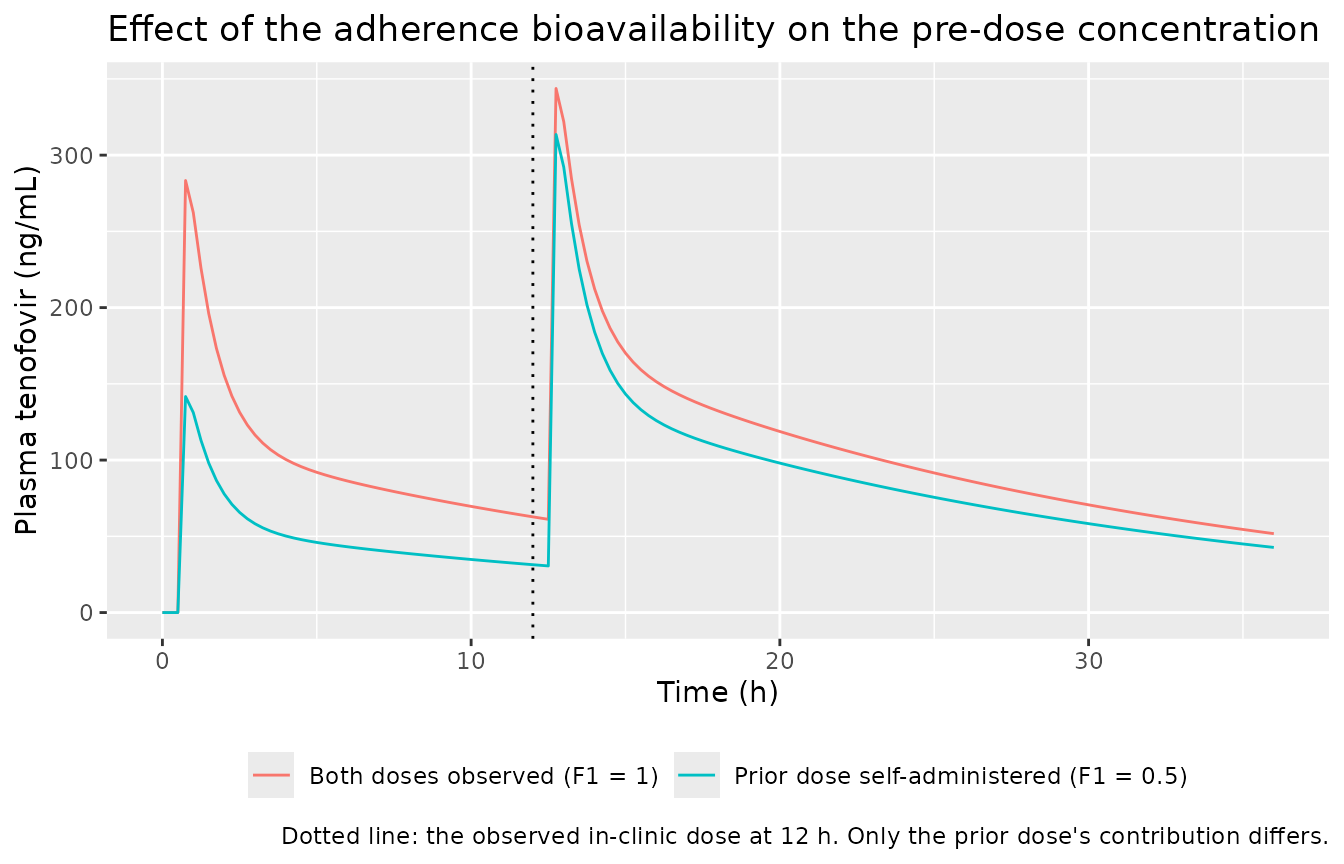


predose <- sim_adh |>
  dplyr::filter(abs(time - 12) < 1e-9) |>
  dplyr::group_by(scenario) |>
  dplyr::summarise(predose = min(Cc) * MW_TFV, .groups = "drop")

knitr::kable(predose, digits = 2,
             caption = "Pre-dose plasma tenofovir immediately before the observed dose.")

Pre-dose plasma tenofovir immediately before the observed dose.
scenario	predose
Both doses observed (F1 = 1)	62.77
Prior dose self-administered (F1 = 0.5)	31.38


stopifnot(
  # Deterministic. With F1 fixed at 0.5 the prior dose contributes exactly half
  # as much residual drug, so the pre-dose concentration must halve; the
  # post-dose profile then converges as the observed dose (F = 1) dominates.
  nrow(predose) == 2L,
  abs(predose$predose[predose$scenario == "Prior dose self-administered (F1 = 0.5)"] /
        predose$predose[predose$scenario == "Both doses observed (F1 = 1)"] - 0.5) < 1e-6
)

Assumptions and deviations

Tenofovir-diphosphate compartment scaling. The paper reports no scaling parameter, volume or S4 for compartment 4, and Supplementary Figure S2 labels that box “PBMC, TFV-DP nm/L” without a volume. The model file therefore applies NONMEM’s default scale of 1 and reads the compartment content directly as the predicted concentration in nmol/L, with the whole amount-to-concentration conversion absorbed into the apparent K24 – which is consistent with the Discussion’s statement that “we modeled only 1 million PBMCs and thus the parameters were apparent in theory”. This reading is not assumed but checked: it reproduces the paper’s own simulated steady-state trough of 49.9 fmol per million cells to within 6% at typical values, a target the reading was not fitted to. No alternative scaling comes within many orders of magnitude.
The fixed adherence variance is read as a variance, not a standard deviation. Methods says the omega distribution was fixed “to a high value, in our case 10”. In NONMEM the $OMEGA block holds variances, so this is encoded as etalfdepot ~ fixed(10) (a log-scale standard deviation of 3.16). The published empirical Bayes range for F1, 0.015-4.17, cannot discriminate between the two readings, because the point of the wide prior is precisely that the estimates are data-driven rather than prior-driven. Nothing in this vignette depends on the choice, since every simulation sets SELFADMIN = 0.
etalka uses the Results text value, not the Table 1 value. Table 1 rounds the final-model between-subject variability on KA to 160.2% CV while the Results text gives 160.16%. The text value is used, as it carries one more significant figure and its companion base-model values in the same sentence match Table 1 exactly. The difference is immaterial (log(1 + CV^2) = 1.27120 versus 1.27156).
Cohort weight distribution. Supplementary Table S1 reports only mean (79.6 kg) and range (43-145 kg), with the median (73 kg) given in Results. The virtual cohort draws from a log-normal centred on the median with sdlog = 0.416 – chosen so the untruncated mean matches 79.6 kg – and truncates to the reported range. The paper publishes no weight histogram, so the shape beyond mean / median / range is an assumption. Truncation at 43 kg removes more of the lower tail than the 145 kg cut removes of the upper, so the realised cohort median runs about 5 kg above the paper’s 73 kg while the realised mean lands on 79.6 kg. That skew has no bearing on any check in this vignette: weight enters the central volume only, and the validated tenofovir-diphosphate quantities are exactly weight-independent (demonstrated in “Weight covariate” above).
The simulated interquartile range of the steady-state trough is wider than the paper’s, for the reason set out in that section: the authors imputed shrunken empirical Bayes estimates for their simulations rather than sampling the published omega. This is recorded as a known deviation and is deliberately excluded from the numeric gate, which is placed on the median.
Only the final model is extracted. Table 1’s Base Model column (identical structure without the weight covariate) is a model-development stage, not a reported final result.
Residual error is proportional-only. Methods describes attempting a combined additive-plus-proportional error model and states that reduction of the residual error model was tested; Table 1 reports only a proportional term per analyte, so the additive terms were dropped.
Covariates screened but not retained – creatinine clearance on K20 and a black / non-black race indicator on clearance – are carried in the model file’s covariatesDataExcluded list for provenance and are not referenced in model().
No observed data are redistributed. The figures replicate the layout and the model-predicted curves of Burns 2015 Figures 2, 4 and 5; the observed points those figures overlay are MTN-001 and Louissaint 2013 participant data and are not reproduced here.
All parameter values come from the paper’s own text, Table 1 and Supplementary Table S1 / Figure S2. No value was digitised from a figure, and no value came from author correspondence or from another publication.