Subcutaneous long-acting risperidone TV-46000 (Perlstein 2022) • nlmixr2lib

Model and source

mod <- readModelDb("Perlstein_2022_risperidone_tv46000")
ui <- rxode2::rxode(mod)
#> ℹ parameter labels from comments will be replaced by 'label()'

Description: Two-compartment population PK model for the risperidone total active moiety (TAM = risperidone + 9-hydroxyrisperidone * 410/426) following subcutaneous TV-46000, a copolymer-based long-acting risperidone suspension, in 97 adults with schizophrenia or schizoaffective disorder from one phase 1 single- and multiple-dose study (Perlstein 2022). Absorption is the paper’s convolution-based prescribed input: a double Weibull release profile that splits the dose between a first release process (shape below 1, front-loaded) and a second, sigmoidal release process, implemented as two parallel depot compartments each emptying with its own Weibull hazard. Allometric body weight on CL/F (exponent 0.75) and V/F (exponent 1) fixed at the 70 kg reference. Exponential inter-individual variability on every structural parameter and a combined additive + proportional residual error. Carries the published Emax dopamine D2 receptor occupancy layer (Kd 10.1 ng/mL) the authors used in their simulations as an algebraic observable. This is the phase 1 TAM model that selected the phase 3 doses; the later pooled parent-metabolite TV-46000 model is modellib(‘Perlstein_2025_risperidone_tv46000’).
Citation: Perlstein I, Merenlender Wagner A, Gomeni R, Lamson M, Harary E, Spiegelstein O, Kalmanczhelyi A, Tiver R, Loupe P, Levi M, Elgart A (2022). Population Pharmacokinetic Modeling and Simulation of TV-46000: A Long-Acting Injectable Formulation of Risperidone. Clin Pharmacol Drug Dev 11(7):865-877. doi:10.1002/cpdd.1078.
Article: https://doi.org/10.1002/cpdd.1078
Supplement: Figures S1-S5 (goodness of fit, all-cohort VPCs, individual fits, all simulated regimens) and the per-cohort sampling schedule. It contains no parameter values, so the model is fully specified by the main text.

TV-46000 is a once-monthly (q1m) or once-every-2-months (q2m) subcutaneous risperidone suspension built on a copolymer delivery technology: the copolymer precipitates on injection, entrapping risperidone in a depot that degrades by hydrolysis. The analysis modelled the total active moiety (TAM), the sum of risperidone and its equipotent metabolite 9-hydroxyrisperidone corrected by molecular weight (TAM = risperidone + 9-OH-risperidone * 410/426, Methods Equation 1), and used the model to choose the phase 3 dose range (50-125 mg q1m, 100-250 mg q2m). The later pooled phase 1 + phase 3 parent-metabolite model of the same product is Perlstein_2025_risperidone_tv46000.

Population

97 of 99 enrolled patients with clinically stable schizophrenia or schizoaffective disorder entered the analysis (two cohort-4 patients were excluded for taking oral risperidone during the TV-46000 period). Mean (SD) age was 44.4 (8.8) years, BMI 28.6 (4.4) kg/m^2, creatinine clearance 115.76 (21.9) mL/min and weight 87 kg; 80% were men and 95.9% Black or African American (Results, Data). Each cohort received 7 days of oral risperidone 2-6 mg/day, a 7-day washout, then TV-46000:

Cohort	TV-46000 regimen	Site
1	50 mg single dose	abdomen
2	75 mg single dose	abdomen
3	100 mg single dose	abdomen
4	150 mg single dose	abdomen
5	225 mg single dose	abdomen
6	75 mg once monthly x 3	abdomen
7	150 mg once monthly x 3	abdomen
8	225 mg single dose	upper arm

Source trace

Element	Value in model	Source
Release function `r(t) = ffexp(-(t/td)^ss) + (1-ff)exp(-(t/td1)^ss1)`	two Weibull-hazard depots	Methods Eq. 3, Figure 2
Input `Dose * (-dr/dt)` into central; 2-compartment disposition	`d/dt(depot)`, `d/dt(depot2)`, `d/dt(central)`, `d/dt(peripheral1)`	Methods Eqs. 2 and 4
`td` = 2.69 week	`lra = log(1/2.69)`	Table 2
`td1` = 3.32 week	`lra2 = log(1/3.32)`	Table 2
`ss` = 0.616	`lgam1 = log(0.616)`	Table 2
`ss1` = 3.66	`lgam2 = log(3.66)`	Table 2
`ff` = 0.511	`logitfrel = logit(0.511)`	Table 2
CL/F = 354 L/week	`lcl = log(354)`	Table 2
V/F = 374 L	`lvc = log(374)`	Table 2
k23 = 1.48 1/week	`lk12 = log(1.48)`	Table 2
k32 = 2.34 1/week	`lk21 = log(2.34)`	Table 2
Allometry `(WT/70)^0.75` on CL, `(WT/70)^1` on V	`e_wt_cl = fixed(0.75)`, `e_wt_vc = fixed(1)`	Methods Eq. 5
IIV variances td 0.163, td1 0.733, ss 0.0247, ss1 0.185, ff 0.115, CL/F 0.117, V/F 0.147, k23 1.41, k32 1.9	`etalra` … `etalk21`	Table 2 Random effect
Proportional 0.152, additive 1.58 ng/mL	`propSd`, `addSd`	Table 2 Residual effect
D2RO = ROmax * Cp / (Kd + Cp), ROmax 100%, Kd 10.1 ng/mL	`emax = fixed(100)`, `lec50 = fixed(log(10.1))`	Methods Eq. 7

Release function

The Results text gives three points on the typical cumulative release curve: about 50% released by 2.6 weeks, 79% by week 4 and 93% by week 8. They test the direction of r(t) (unreleased, not released, fraction) and the time unit. The two depots of the packaged model hold exactly the unreleased dose, so their typical-value contents after a single injection must reproduce Equation 3.

th <- ui$theta
ra <- exp(th[["lra"]]); ra2 <- exp(th[["lra2"]])
gam1 <- exp(th[["lgam1"]]); gam2 <- exp(th[["lgam2"]])
frel <- plogis(th[["logitfrel"]])

ev_rel <- et(amt = 100, cmt = "depot") |>
  et(amt = 100, cmt = "depot2") |>
  et(c(2.6, 4, 8))
rel <- rxSolve(rxode2::zeroRe(mod), ev_rel, params = c(WT = 70)) |>
  as.data.frame() |>
  mutate(
    released_model = 1 - (depot + depot2) / 100,
    released_eq3 = 1 - (frel * exp(-(ra * time)^gam1) + (1 - frel) * exp(-(ra2 * time)^gam2)),
    released_paper = c(0.50, 0.79, 0.93)
  )
#> ℹ parameter labels from comments will be replaced by 'label()'
#> ℹ omega/sigma items treated as zero: 'etalra', 'etalra2', 'etalgam1', 'etalgam2', 'etalogitfrel', 'etalcl', 'etalvc', 'etalk12', 'etalk21'
knitr::kable(
  rel |>
    select(time, released_model, released_eq3, released_paper) |>
    rename(
      "Time (week)" = time,
      "Released, model depots" = released_model,
      "Released, Equation 3" = released_eq3,
      "Released, Results text" = released_paper
    ),
  digits = 3
)

Time (week)	Released, model depots	Released, Equation 3	Released, Results text
2.6	0.483	0.483	0.50
4.0	0.790	0.790	0.79
8.0	0.928	0.928	0.93

# Same parameters, closed form vs ODE: pure numerical error.
stopifnot(all(abs(rel$released_model - rel$released_eq3) < 1e-4))
# Against the rounded percentages printed in the Results.
stopifnot(all(abs(rel$released_model - rel$released_paper) < 0.02))

Virtual cohort

The paper reports mean weight (87 kg) but not its spread. Weights are drawn from a normal distribution with mean 87 kg and an assumed SD of 15 kg (consistent with the BMI SD of 4.4 kg/m^2), truncated to 55-140 kg.

n_per_arm <- 200
make_cohort <- function(n, seed) {
  set.seed(seed)
  wt <- rnorm(n * 3, 87, 15)
  wt <- wt[wt >= 55 & wt <= 140][seq_len(n)]
  data.frame(id = seq_len(n), WT = wt)
}

# One TV-46000 injection = one record on each depot with the same amount.
inject <- function(ids, times, amt) {
  expand.grid(id = ids, time = times, cmt = c("depot", "depot2"), stringsAsFactors = FALSE) |>
    mutate(amt = amt, evid = 1L)
}
observe <- function(ids, times) {
  expand.grid(id = ids, time = times) |>
    mutate(cmt = "central", amt = NA_real_, evid = 0L)
}

Visual predictive checks (Figure 3)

arms <- tibble::tribble(
  ~panel, ~label, ~amt, ~n_dose, ~t_end,
  "A", "75 mg single dose (cohort 2)", 75, 1, 12,
  "B", "150 mg single dose (cohort 4)", 150, 1, 15,
  "C", "75 mg once monthly x 3 (cohort 6)", 75, 3, 20,
  "D", "150 mg once monthly x 3 (cohort 7)", 150, 3, 20
)
obs_grid <- sort(unique(c(seq(0, 1, by = 1 / 7), seq(1, 20, by = 0.25))))

rxode2::rxSetSeed(2022)
sim_vpc <- bind_rows(lapply(seq_len(nrow(arms)), function(i) {
  a <- arms[i, ]
  cohort <- make_cohort(n_per_arm, seed = 100 + i)
  ev <- bind_rows(
    inject(cohort$id, 4 * (seq_len(a$n_dose) - 1), a$amt),
    observe(cohort$id, obs_grid[obs_grid <= a$t_end])
  ) |>
    left_join(cohort, by = "id") |>
    arrange(id, time, desc(evid))
  rxSolve(mod, ev, returnType = "data.frame") |>
    mutate(panel = a$panel, label = a$label)
}))
#> ℹ parameter labels from comments will be replaced by 'label()'

vpc_summary <- sim_vpc |>
  group_by(panel, label, time) |>
  summarise(
    p05 = quantile(Cc, 0.05), p50 = median(Cc), p95 = quantile(Cc, 0.95),
    .groups = "drop"
  )

# Median curves read by the maintainers from Figure 3 (approximate, +/- 2 ng/mL).
fig3 <- tibble::tribble(
  ~panel, ~time, ~median_fig,
  "A", 1, 14, "A", 2, 13.5, "A", 4, 11, "A", 6, 7, "A", 8, 4.5, "A", 10, 3, "A", 12, 2.5,
  "B", 1, 28, "B", 2, 30, "B", 3, 28, "B", 5, 17, "B", 7.5, 10, "B", 10, 6, "B", 15, 3,
  "C", 4, 11, "C", 5.5, 23, "C", 8, 15, "C", 9, 27, "C", 15, 7, "C", 20, 3,
  "D", 4, 19, "D", 5.5, 47, "D", 8, 29, "D", 9, 55, "D", 15, 15, "D", 20, 6
) |>
  left_join(distinct(arms, panel, label), by = "panel")

ggplot(vpc_summary, aes(time)) +
  geom_ribbon(aes(ymin = p05, ymax = p95), fill = "lightblue", alpha = 0.6) +
  geom_line(aes(y = p50), colour = "blue", linewidth = 0.8) +
  geom_point(data = fig3, aes(y = median_fig), shape = 4, size = 2) +
  facet_wrap(~label, scales = "free_x") +
  labs(
    x = "Time (week)", y = "Total active moiety (ng/mL)",
    caption = paste(
      "Replicates Figure 3 of Perlstein 2022: simulated median and 90% prediction interval.",
      "Crosses: the published median curve, read from the figure."
    )
  )

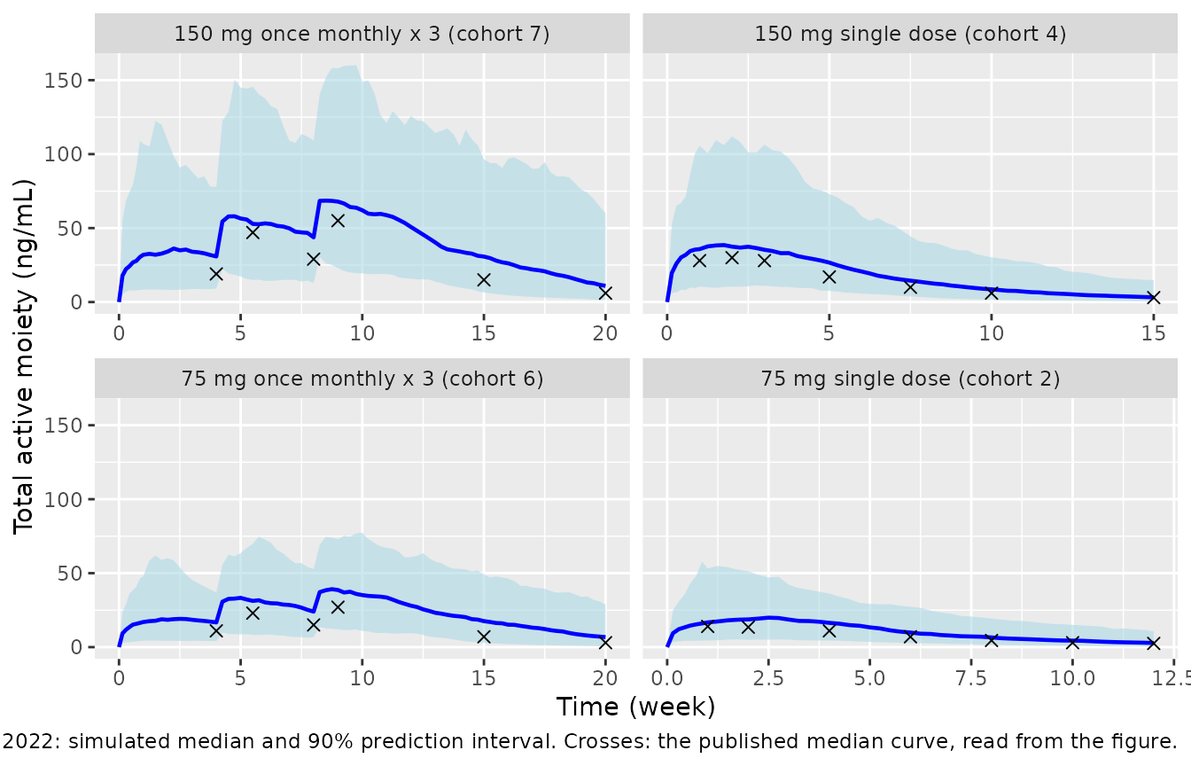
The simulated medians sit above the published VPC medians at every time point, and the gap widens after the peak:

vpc_ratio <- fig3 |>
  left_join(vpc_summary, by = c("panel", "label", "time")) |>
  mutate(ratio = p50 / median_fig)
knitr::kable(
  vpc_ratio |>
    select(label, time, median_fig, p50, ratio) |>
    rename(
      "Arm" = label, "Time (week)" = time,
      "Figure 3 median (ng/mL)" = median_fig,
      "Simulated median (ng/mL)" = p50,
      "Simulated / Figure 3" = ratio
    ),
  digits = 2
)

Arm	Time (week)	Figure 3 median (ng/mL)	Simulated median (ng/mL)	Simulated / Figure 3
75 mg single dose (cohort 2)	1.0	14.0	16.74	1.20
75 mg single dose (cohort 2)	2.0	13.5	18.75	1.39
75 mg single dose (cohort 2)	4.0	11.0	16.40	1.49
75 mg single dose (cohort 2)	6.0	7.0	9.87	1.41
75 mg single dose (cohort 2)	8.0	4.5	6.54	1.45
75 mg single dose (cohort 2)	10.0	3.0	4.41	1.47
75 mg single dose (cohort 2)	12.0	2.5	2.83	1.13
150 mg single dose (cohort 4)	1.0	28.0	35.78	1.28
150 mg single dose (cohort 4)	2.0	30.0	37.46	1.25
150 mg single dose (cohort 4)	3.0	28.0	35.33	1.26
150 mg single dose (cohort 4)	5.0	17.0	26.67	1.57
150 mg single dose (cohort 4)	7.5	10.0	14.48	1.45
150 mg single dose (cohort 4)	10.0	6.0	8.60	1.43
150 mg single dose (cohort 4)	15.0	3.0	3.24	1.08
75 mg once monthly x 3 (cohort 6)	4.0	11.0	16.71	1.52
75 mg once monthly x 3 (cohort 6)	5.5	23.0	31.26	1.36
75 mg once monthly x 3 (cohort 6)	8.0	15.0	24.01	1.60
75 mg once monthly x 3 (cohort 6)	9.0	27.0	38.62	1.43
75 mg once monthly x 3 (cohort 6)	15.0	7.0	17.57	2.51
75 mg once monthly x 3 (cohort 6)	20.0	3.0	6.77	2.26
150 mg once monthly x 3 (cohort 7)	4.0	19.0	30.82	1.62
150 mg once monthly x 3 (cohort 7)	5.5	47.0	52.83	1.12
150 mg once monthly x 3 (cohort 7)	8.0	29.0	43.74	1.51
150 mg once monthly x 3 (cohort 7)	9.0	55.0	67.90	1.23
150 mg once monthly x 3 (cohort 7)	15.0	15.0	30.75	2.05
150 mg once monthly x 3 (cohort 7)	20.0	6.0	10.95	1.82

See the Errata section: these ratios, together with Table 3 below, indicate that the clearance printed in Table 2 is about 1.4-fold lower than the clearance the authors’ own figures and simulations were produced with.

Steady-state exposure (Table 3)

Table 3 reports the median steady-state AUC over the dosing interval for four q1m and four q2m regimens. Every regimen is simulated for 64 weeks (16 q1m or 8 q2m injections) so that the last interval is close to steady state even for patients with a slow peripheral return rate k21; PKNCA computes AUC over that interval, converted from ngweek/mL to the ngh/mL of the table. All arms share the same virtual patients and the same random effects, so differences between arms come from the regimen alone.

ss_arms <- tibble::tribble(
  ~treatment, ~amt, ~tau,
  "50 mg q1m", 50, 4, "75 mg q1m", 75, 4, "100 mg q1m", 100, 4, "125 mg q1m", 125, 4,
  "100 mg q2m", 100, 8, "150 mg q2m", 150, 8, "200 mg q2m", 200, 8, "250 mg q2m", 250, 8
)
t_total <- 64
ss_arms$n_inj <- t_total / ss_arms$tau

ss_cohort <- make_cohort(n_per_arm, seed = 7)
ss_ev <- lapply(seq_len(nrow(ss_arms)), function(i) {
  a <- ss_arms[i, ]
  t_last <- a$tau * (a$n_inj - 1)
  grid <- sort(unique(c(0, seq(t_last, t_last + a$tau, by = 0.05))))
  bind_rows(
    inject(ss_cohort$id, a$tau * (seq_len(a$n_inj) - 1), a$amt),
    observe(ss_cohort$id, grid)
  ) |>
    left_join(ss_cohort, by = "id") |>
    arrange(id, time, desc(evid)) |>
    mutate(treatment = a$treatment)
})
sim_ss <- bind_rows(lapply(ss_ev, function(ev) {
  # Re-seeding before every arm gives each virtual patient the same etas in
  # every arm.
  rxode2::rxSetSeed(20221)
  rxSolve(mod, select(ev, -treatment), returnType = "data.frame") |>
    mutate(treatment = ev$treatment[1])
}))

conc_df <- sim_ss |>
  filter(!is.na(Cc)) |>
  select(id, time, Cc, treatment)
dose_df <- bind_rows(ss_ev) |>
  filter(evid == 1, cmt == "depot") |>
  select(id, time, amt, treatment)

intervals <- ss_arms |>
  transmute(
    treatment,
    start = t_total - tau, end = t_total,
    auclast = TRUE, cmax = TRUE, cmin = TRUE
  )

nca <- PKNCA::pk.nca(PKNCA::PKNCAdata(
  PKNCA::PKNCAconc(conc_df, Cc ~ time | treatment + id),
  PKNCA::PKNCAdose(dose_df, amt ~ time | treatment + id),
  intervals = intervals
))
nca_res <- as.data.frame(nca$result) |>
  mutate(PPORRES = ifelse(PPTESTCD == "auclast", PPORRES * 168, PPORRES))

published <- tibble::tribble(
  ~treatment, ~auclast,
  "50 mg q1m", 14076, "75 mg q1m", 21136, "100 mg q1m", 28607, "125 mg q1m", 34402,
  "100 mg q2m", 29419, "150 mg q2m", 44243, "200 mg q2m", 58508, "250 mg q2m", 73558
)

cmp <- nlmixr2lib::ncaComparisonTable(
  simulated = nca_res |> filter(PPTESTCD == "auclast"),
  reference = published,
  by = "treatment",
  units = c(auclast = "ng*h/mL"),
  tolerance_pct = 20
)
knitr::kable(
  cmp,
  caption = "Simulated vs. published steady-state AUC over the dosing interval (Perlstein 2022 Table 3). * differs from reference by >20%."
)

Simulated vs. published steady-state AUC over the dosing interval (Perlstein 2022 Table 3). * differs from reference by >20%.
NCA parameter	treatment	Reference	Simulated	% diff
AUClast (ng*h/mL)	50 mg q1m	14100	18300	+30.2%*
AUClast (ng*h/mL)	75 mg q1m	21100	27500	+30.1%*
AUClast (ng*h/mL)	100 mg q1m	28600	36700	+28.2%*
AUClast (ng*h/mL)	125 mg q1m	34400	45800	+33.2%*
AUClast (ng*h/mL)	100 mg q2m	29400	37300	+26.6%*
AUClast (ng*h/mL)	150 mg q2m	44200	55900	+26.3%*
AUClast (ng*h/mL)	200 mg q2m	58500	74500	+27.3%*
AUClast (ng*h/mL)	250 mg q2m	73600	93100	+26.6%*

Every row is starred: the simulated steady-state AUC is 26-33% above the published value. At steady state AUCtau = Dose / CL for any release function with complete release, so this comparison isolates the clearance and is unaffected by the release parameters and the multiple-dose approximation. For a typical 87 kg patient, Dose / CL for 100 mg q1m is 40,300 ng*h/mL, 1.41 times the printed 28,607; the simulated cohort median sits a little lower because patients who draw a slow peripheral return rate are still filling the peripheral compartment after 64 weeks. The parts of Table 3 that do not depend on the clearance value are reproduced:

auc_med <- nca_res |>
  filter(PPTESTCD == "auclast") |>
  group_by(treatment) |>
  summarise(auc = median(PPORRES), .groups = "drop") |>
  left_join(ss_arms, by = "treatment") |>
  left_join(published |> rename(auc_pub = auclast), by = "treatment") |>
  mutate(
    daily_sim = auc / (7 * tau), daily_pub = auc_pub / (7 * tau),
    ratio = auc / auc_pub
  )

pair <- tibble::tibble(q1m = c("50 mg q1m", "75 mg q1m", "100 mg q1m", "125 mg q1m"),
                       q2m = c("100 mg q2m", "150 mg q2m", "200 mg q2m", "250 mg q2m"))
pair_chk <- pair |>
  mutate(
    sim = auc_med$daily_sim[match(q2m, auc_med$treatment)] / auc_med$daily_sim[match(q1m, auc_med$treatment)],
    pub = auc_med$daily_pub[match(q2m, auc_med$treatment)] / auc_med$daily_pub[match(q1m, auc_med$treatment)]
  )
knitr::kable(
  pair_chk |>
    rename(
      "q1m regimen" = q1m, "q2m regimen" = q2m,
      "Daily AUC ratio q2m/q1m, simulated" = sim,
      "Daily AUC ratio q2m/q1m, Table 3" = pub
    ),
  digits = 3
)

q1m regimen	q2m regimen	Daily AUC ratio q2m/q1m, simulated	Daily AUC ratio q2m/q1m, Table 3
50 mg q1m	100 mg q2m	1.016	1.045
75 mg q1m	150 mg q2m	1.016	1.047
100 mg q1m	200 mg q2m	1.016	1.023
125 mg q1m	250 mg q2m	1.016	1.069


stopifnot(
  # Clearance-free: equal daily dose gives equal daily exposure, as Table 3 shows.
  all(abs(pair_chk$sim / pair_chk$pub - 1) < 0.08),
  # The documented Table 2 vs Table 3 clearance discrepancy (see Errata). If this
  # fails, the model's clearance has changed and the Errata must be revisited.
  median(auc_med$ratio) > 1.15, median(auc_med$ratio) < 1.6
)

Simulated profiles and D2 receptor occupancy (Figures 4 and 5)

rxode2::rxSetSeed(20222)
d2_arms <- tibble::tribble(
  ~label, ~amt, ~tau, ~n_dose,
  "75 mg q1m", 75, 4, 6, "150 mg q2m", 150, 8, 3,
  "100 mg q1m", 100, 4, 6, "200 mg q2m", 200, 8, 3
)
d2_cohort <- make_cohort(n_per_arm, seed = 11)
sim_d2 <- bind_rows(lapply(seq_len(nrow(d2_arms)), function(i) {
  a <- d2_arms[i, ]
  ev <- bind_rows(
    inject(d2_cohort$id, a$tau * (seq_len(a$n_dose) - 1), a$amt),
    observe(d2_cohort$id, seq(0, 24, by = 0.1))
  ) |>
    left_join(d2_cohort, by = "id") |>
    arrange(id, time, desc(evid))
  rxSolve(mod, ev, returnType = "data.frame") |>
    mutate(label = a$label)
}))
d2_sum <- sim_d2 |>
  group_by(label, time) |>
  summarise(
    across(c(Cc, D2RO), list(
      p025 = ~ quantile(.x, 0.025), p05 = ~ quantile(.x, 0.05), p50 = median,
      p95 = ~ quantile(.x, 0.95), p975 = ~ quantile(.x, 0.975)
    )),
    .groups = "drop"
  )

ggplot(filter(d2_sum, label %in% c("100 mg q1m", "200 mg q2m")), aes(time)) +
  geom_ribbon(aes(ymin = Cc_p05, ymax = Cc_p95), fill = "lightblue", alpha = 0.6) +
  geom_line(aes(y = Cc_p50), colour = "blue") +
  scale_y_log10() +
  facet_wrap(~label, ncol = 1) +
  labs(
    x = "Time since first injection (week)", y = "Total active moiety (ng/mL)",
    caption = "Replicates the TV-46000 part of Figure 4 of Perlstein 2022 (median and 90% interval; oral lead-in not simulated)."
  )
#> Warning in scale_y_log10(): log-10 transformation introduced infinite values.
#> log-10 transformation introduced infinite values.
#> log-10 transformation introduced infinite values.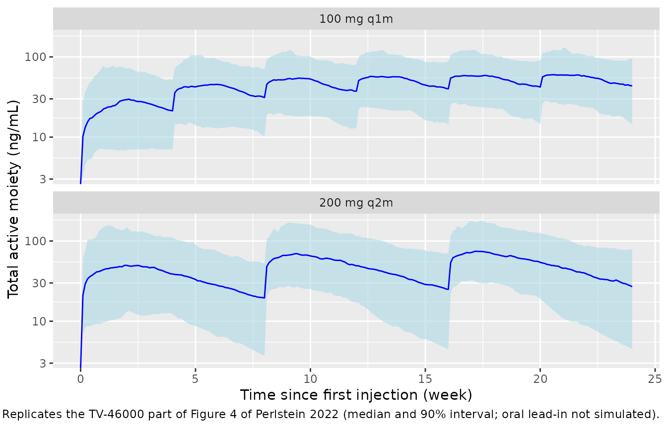


ggplot(filter(d2_sum, label %in% c("75 mg q1m", "150 mg q2m")), aes(time)) +
  geom_ribbon(aes(ymin = D2RO_p025, ymax = D2RO_p975), fill = "pink", alpha = 0.5) +
  geom_ribbon(aes(ymin = D2RO_p05, ymax = D2RO_p95), fill = "orchid", alpha = 0.5) +
  geom_line(aes(y = D2RO_p50), colour = "darkblue") +
  geom_hline(yintercept = c(20, 60, 80), linetype = "dashed") +
  facet_wrap(~label) +
  labs(
    x = "Time since first injection (week)", y = "D2 receptor occupancy (%)",
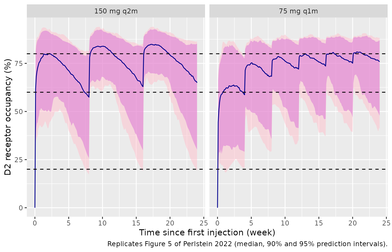
    caption = "Replicates Figure 5 of Perlstein 2022 (median, 90% and 95% prediction intervals)."
  )

Multiple-dose approximation

The paper’s convolution input superposes every injection on its own clock. The packaged model holds all injections in one pair of Weibull depots, whose hazard restarts at each new injection, so drug still left from an earlier injection is released on the new injection’s clock. The size of that approximation is checked here against an exact reference model with a separate depot pair for every injection, at typical values for a 70 kg patient.

n_ref <- 8
depot_code <- vapply(seq_len(n_ref), function(k) {
  sprintf(paste(
    "h1_%1$d <- gam1 * ra * (ra * max(tad0(da_%1$d), 1e-6))^(gam1 - 1)",
    "h2_%1$d <- gam2 * ra2 * (ra2 * max(tad0(db_%1$d), 1e-6))^(gam2 - 1)",
    "d/dt(da_%1$d) <- -h1_%1$d * da_%1$d",
    "d/dt(db_%1$d) <- -h2_%1$d * db_%1$d",
    "f(da_%1$d) <- frel",
    "f(db_%1$d) <- 1 - frel",
    sep = "\n"
  ), k)
}, character(1))
input <- paste(sprintf("h1_%1$d * da_%1$d + h2_%1$d * db_%1$d", seq_len(n_ref)), collapse = " + ")
ref_mod <- rxode2::rxode2(paste(c(
  depot_code,
  sprintf("d/dt(central) <- %s - kel * central - k12 * central + k21 * peripheral1", input),
  "d/dt(peripheral1) <- k12 * central - k21 * peripheral1",
  "Cc <- 1000 * central / vc"
), collapse = "\n"))

typ <- c(
  ra = ra, ra2 = ra2, gam1 = gam1, gam2 = gam2, frel = frel,
  kel = exp(th[["lcl"]]) / exp(th[["lvc"]]), vc = exp(th[["lvc"]]),
  k12 = exp(th[["lk12"]]), k21 = exp(th[["lk21"]])
)

approx_chk <- bind_rows(lapply(c(4, 8), function(tau) {
  grid <- seq(0, n_ref * tau, by = 0.05)
  ev_ref <- et(grid)
  for (k in seq_len(n_ref)) {
    ev_ref <- ev_ref |>
      et(time = (k - 1) * tau, amt = 100, cmt = sprintf("da_%d", k)) |>
      et(time = (k - 1) * tau, amt = 100, cmt = sprintf("db_%d", k))
  }
  exact <- as.data.frame(rxSolve(ref_mod, typ, ev_ref))
  ev_pkg <- et(grid) |>
    et(amt = 100, cmt = "depot", ii = tau, addl = n_ref - 1) |>
    et(amt = 100, cmt = "depot2", ii = tau, addl = n_ref - 1)
  pkg <- as.data.frame(rxSolve(rxode2::zeroRe(mod), ev_pkg, params = c(WT = 70)))
  last <- exact$time >= (n_ref - 1) * tau
  tibble::tibble(
    regimen = sprintf("100 mg every %d weeks", tau),
    max_abs_pct_diff = max(abs(pkg$Cc[exact$time > 0] / exact$Cc[exact$time > 0] - 1)) * 100,
    cmax_ss_exact = max(exact$Cc[last]), cmax_ss_model = max(pkg$Cc[last]),
    cmin_ss_exact = min(exact$Cc[last]), cmin_ss_model = min(pkg$Cc[last])
  )
}))
#> ℹ parameter labels from comments will be replaced by 'label()'
#> ℹ omega/sigma items treated as zero: 'etalra', 'etalra2', 'etalgam1', 'etalgam2', 'etalogitfrel', 'etalcl', 'etalvc', 'etalk12', 'etalk21'
#> ℹ parameter labels from comments will be replaced by 'label()'
#> ℹ omega/sigma items treated as zero: 'etalra', 'etalra2', 'etalgam1', 'etalgam2', 'etalogitfrel', 'etalcl', 'etalvc', 'etalk12', 'etalk21'
knitr::kable(
  approx_chk |>
    rename(
      "Regimen" = regimen, "Max |difference| over time (%)" = max_abs_pct_diff,
      "Cmax,ss exact" = cmax_ss_exact, "Cmax,ss model" = cmax_ss_model,
      "Cmin,ss exact" = cmin_ss_exact, "Cmin,ss model" = cmin_ss_model
    ),
  digits = 2
)

Regimen	Max \|difference\| over time (%)	Cmax,ss exact	Cmax,ss model	Cmin,ss exact	Cmin,ss model
100 mg every 4 weeks	8.14	82.56	84.8	64.15	63.31
100 mg every 8 weeks	7.79	55.31	55.1	12.40	11.54

stopifnot(all(approx_chk$max_abs_pct_diff < 12))

Concentrations differ from exact superposition by less than about 8% at any time, and steady-state AUC is identical because every injection is still fully released. For a regimen where that matters, give each injection its own depot pair as in the reference model above.

Assumptions and deviations

Clearance in Table 2 vs the paper’s own figures and simulations (unresolved). With CL/F = 354 L/week as printed, the simulated steady-state AUC is 26-33% above every Table 3 value (1.41-fold for a typical 87 kg patient), and the simulated Figure 3 medians sit 1.1-1.6 times above the published single-dose medians and up to 2.5 times above the late multiple-dose ones. Neither discrepancy can come from the release function or the virtual weights: steady-state AUC is Dose / CL exactly, and reaching Table 3 by weight alone would need a typical patient of about 140 kg against a study mean of 87 kg. A clearance of about 1.4 x 354 = 496 L/week closes the typical-patient Table 3 gap and brings the single-dose Figure 3 medians into line (shown below), which points to a reporting error in the Table 2 clearance, but the paper states no other value and has no erratum (checked 2026-10-03). The model therefore carries the printed 354 L/week, and users who need the paper’s simulated exposures should be aware of the difference. The later pooled TV-46000 model (Perlstein_2025_risperidone_tv46000) implies a typical TAM clearance of about 4.2 L/h (about 710 L/week), which is also above 354 L/week.

rxode2::rxSetSeed(2022)
sens <- bind_rows(lapply(c(1, 2), function(i) {
  a <- arms[i, ]
  cohort <- make_cohort(n_per_arm, seed = 100 + i)
  ev <- bind_rows(
    inject(cohort$id, 0, a$amt),
    observe(cohort$id, unique(fig3$time[fig3$panel == a$panel]))
  ) |>
    left_join(cohort, by = "id") |>
    arrange(id, time, desc(evid))
  bind_rows(
    rxSolve(mod, ev, returnType = "data.frame") |> mutate(cl_case = "Table 2 CL/F (354 L/week)"),
    rxSolve(mod |> ini(lcl = log(354 * 1.4)), ev, returnType = "data.frame") |>
      mutate(cl_case = "Diagnostic only: 1.4 x CL/F")
  ) |>
    mutate(panel = a$panel)
})) |>
  group_by(cl_case, panel, time) |>
  summarise(p50 = median(Cc), .groups = "drop") |>
  inner_join(fig3, by = c("panel", "time")) |>
  group_by(cl_case) |>
  summarise(median_ratio_to_figure3 = median(p50 / median_fig), .groups = "drop")
#> ℹ parameter labels from comments will be replaced by 'label()'
#> ℹ change initial estimate of `lcl` to `6.20576914975499`
#> ℹ parameter labels from comments will be replaced by 'label()'
#> ℹ change initial estimate of `lcl` to `6.20576914975499`
knitr::kable(
  sens |>
    rename("Clearance" = cl_case, "Median of simulated / Figure 3 median (panels A, B)" = median_ratio_to_figure3),
  digits = 2
)

Clearance	Median of simulated / Figure 3 median (panels A, B)
Diagnostic only: 1.4 x CL/F	0.93
Table 2 CL/F (354 L/week)	1.43

ff on the logit scale. The paper puts a log-normal random effect on the first-process fraction (variance 0.115). Applied to ff = 0.511, that gives ff > 1 (and a negative second-process fraction) for about 2.4% of patients. The model holds ff on the logit scale and converts the variance by the delta method, 0.115 / (1 - 0.511)^2 = 0.481, matching the typical value and the local spread while keeping both fractions in (0, 1). The Results text’s “ff = 0.55%” is a typo for Table 2’s 0.511.
IIV on CL/F and V/F, not kel. The Methods list IIV on kel, but Table 2 reports IIV on CL/F and V/F; the model follows Table 2.
Omega and residual scales. Table 2 random effects are taken as NONMEM OMEGA variances; its “SE,%” column is the SE multiplied by 100 (for example 0.163 x 45.3% = 0.0738, printed 7.38). The proportional (0.152) and additive (1.58 ng/mL) residual errors are taken as standard deviations of a combined error model, since the table reports a single epsilon shrinkage for the pair.
Weight distribution. Only the mean weight (87 kg) is reported; the virtual cohorts use an assumed SD of 15 kg.
Multiple doses. One depot pair carries all injections; see the multiple-dose approximation section for its size.
Parameter names. The paper’s ss / ss1 (sigmoidicity) are gam1 / gam2 and its td / td1 are expressed as rates ra = 1/td, ra2 = 1/td1. The name ss cannot be used in an rxode2 model because it is the steady-state event flag. The paper’s peripheral rate constants k23 / k32 are k12 / k21.
Covariates screened but not retained (age, injection site, BMI, creatinine clearance, sex, race) are recorded in covariatesDataExcluded.