Tamsulosin (Tsuda 2010)
Source:vignettes/articles/Tsuda_2010_tamsulosin.Rmd
Tsuda_2010_tamsulosin.RmdModel and source
- Citation: Tsuda Y, Tatami S, Yamamura N, Tadayasu Y, Sarashina A, Liesenfeld K-H, Staab A, Schaefer H-G, Ieiri I, Higuchi S. Population pharmacokinetics of tamsulosin hydrochloride in paediatric patients with neuropathic and non-neuropathic bladder. British Journal of Clinical Pharmacology. 2010;70(1):88-101. doi:10.1111/j.1365-2125.2010.03662.x
- Description: One-compartment population PK model for oral modified-release tamsulosin hydrochloride in paediatric patients (2-16 years) with neuropathic and non-neuropathic bladder (Tsuda 2010), with first-order absorption after a lag time, allometric (WT/70)^0.75 on apparent clearance and (WT/70)^1 on apparent central volume (allometric exponents fixed at theory values), a power-form alpha-1-acid glycoprotein (AAG/20 uM) effect on both CL/F and V/F, correlated inter-individual variability on CL/F and V/F, independent IIV on ka, and a combined additive + proportional residual error.
- Article: https://doi.org/10.1111/j.1365-2125.2010.03662.x
Population
The model was developed from 1082 plasma tamsulosin HCl concentrations from 189 paediatric patients pooled across three clinical trials (Tsuda 2010 Table 1A): trial 1 (phase I single dose in non-neurogenic bladder, n = 45), trial 2 (phase II long-term safety / efficacy in neurogenic bladder with a PK sub-study, n = 29), and trial 3 (phase IIb / III double-blind randomised placebo-controlled dose-ranging trial in neurogenic bladder, n = 115). Age range was 2-16 years (median 8); body weight 12.1-92.2 kg (median 25.0); 44% female; race mix in step 2 was White 46%, Asian 44%, Black or African American 3%, American Indian or Alaska Native 7% (Tsuda 2010 Table 2). Trials 2 and 3 administered the modified release capsule contents sprinkled over applesauce or yogurt; a biowaiver covered this paediatric administration based on in vitro dissolution comparison with the adult commercial product. Per-trial dosing schemes (Tsuda 2010 Table 1B for trial 1, Table 1C for trials 2 and 3) ranged from 0.025 to 0.8 mg once daily across weight bands. The PK base model was developed on the frequent-sampling data from trials 1 and 2 (step 1, n = 74) and the covariate model added the sparse trial 3 data (step 2, n = 189).
The same information is available programmatically via
readModelDb("Tsuda_2010_tamsulosin")$population.
Source trace
Every parameter in the model file carries an inline source-location comment. The table below collects the entries in one place.
| Equation / parameter | Value | Source location |
|---|---|---|
lcl (CL/F at WT 70 kg, AAG 20 uM) |
2.28 L/h | Table 3, row ‘CL/F (l h-1)’ |
e_aag_cl (AAG/20 exponent on CL/F) |
-0.844 | Table 3, row ‘theta_AAG_CL’ |
lvc (V/F at WT 70 kg, AAG 20 uM) |
37.5 L | Table 3, row ‘V/F (l)’ |
e_aag_vc (AAG/20 exponent on V/F) |
-0.663 | Table 3, row ‘theta_AAG_V’ |
lka (ka) |
0.368 1/h | Table 3, row ‘Ka (h-1)’ |
ltlag (absorption lag) |
0.957 h | Table 3, row ‘ALAG1 (h)’ |
e_wt_cl (allometric exponent on CL/F) |
0.75 (fixed) | Table 3 structural equation; Methods Step 1; Results Step 2 (CI for the estimated 0.768 included 0.75 -> fixed) |
e_wt_vc (allometric exponent on V/F) |
1.0 (fixed) | Table 3 structural equation; Methods Step 1; Results Step 2 (CI for the estimated 0.807 included 1.0 -> fixed) |
| Reference weight 70 kg | - | Table 3 structural equation ‘(WT/70)’ |
| Reference AAG 20 uM | - | Table 3 structural equation ‘(AAG/20.0)’ |
| IIV CL/F (54.4%; omega^2 = 0.544^2 = 0.2959) | 54.4% CV | Table 3, row ‘IIV in CL/F’ |
| IIV V/F (61.2%; omega^2 = 0.612^2 = 0.3745) | 61.2% CV | Table 3, row ‘IIV in V/F’ |
| IIV ka (117%; omega^2 = 1.17^2 = 1.3689) | 117% CV | Table 3, row ‘IIV in Ka’ |
| Cov(CL/F, V/F) = 0.238 (correlation 0.715) | 0.238 | Table 3, row ‘Cov_V/CL’ |
| Proportional residual error (28.4%; propSd 0.284) | 28.4% CV | Table 3, row ‘Proportional residual variability (CV%)’ |
| Additive residual error (0.178 ng/mL) | 0.178 ng/mL | Table 3, row ‘Additive residual variability (SD ng ml-1)’ |
| Structural model: 1 cmt + FOA + lag time | - | Methods ‘Population pharmacokinetic modelling’ paragraph 1; Results ‘Step 1’ |
| Combined residual error Y = Yhat + Yhat*eps1 + eps2 | - | Methods ‘Population pharmacokinetic modelling’ paragraph 1; Table 3 header |
Virtual cohort
The original observed data are not publicly available. The virtual cohorts below reproduce the simulation scenarios of Tsuda 2010 Figure 4 (effect of body weight and AAG on steady-state Cmax and AUC) and Figure 5 (weight-based dosing scheme in paediatrics vs. adult NCA at 0.4 mg).
set.seed(20100501)

n_per_band <- 200L

make_cohort <- function(n, wt, aag, label, id_offset = 0L) {
  tibble(
    id    = id_offset + seq_len(n),
    WT    = wt,
    AAG   = aag,
    cohort = label
  )
}

# Figure 4 left panel -- four body weights at the cohort-median AAG = 20 uM
fig4_wt <- bind_rows(
  make_cohort(n_per_band, wt = 12.5, aag = 20, label = "12.5 kg", id_offset = 0L),
  make_cohort(n_per_band, wt = 25.0, aag = 20, label = "25.0 kg", id_offset = 1L * n_per_band),
  make_cohort(n_per_band, wt = 50.0, aag = 20, label = "50.0 kg", id_offset = 2L * n_per_band),
  make_cohort(n_per_band, wt = 70.0, aag = 20, label = "70.0 kg", id_offset = 3L * n_per_band)
) |>
  mutate(cohort = factor(cohort, levels = c("12.5 kg", "25.0 kg", "50.0 kg", "70.0 kg")))
stopifnot(!anyDuplicated(fig4_wt$id))

# Figure 4 right panel -- four AAG concentrations at the cohort-median WT = 25 kg
fig4_aag <- bind_rows(
  make_cohort(n_per_band, wt = 25, aag = 10, label = "AAG 10 uM", id_offset = 0L),
  make_cohort(n_per_band, wt = 25, aag = 20, label = "AAG 20 uM", id_offset = 1L * n_per_band),
  make_cohort(n_per_band, wt = 25, aag = 30, label = "AAG 30 uM", id_offset = 2L * n_per_band),
  make_cohort(n_per_band, wt = 25, aag = 40, label = "AAG 40 uM", id_offset = 3L * n_per_band)
) |>
  mutate(cohort = factor(cohort, levels = c("AAG 10 uM", "AAG 20 uM", "AAG 30 uM", "AAG 40 uM")))
stopifnot(!anyDuplicated(fig4_aag$id))
Simulation
Tamsulosin HCl is dosed once daily; steady state is reached by the fifth day of dosing (Tsuda 2010 Discussion paragraph 5). The simulations below dose 10 days of 0.1 mg once daily (the paper’s Figure 4 dose) and characterise the day-10 dosing interval as the steady-state interval.
build_events <- function(demo, dose_mg, n_doses = 10, tau = 24,
                          obs_grid = seq(0, n_doses * tau, by = 0.25)) {
  doses <- demo |>
    mutate(amt  = dose_mg,
           evid = 1L,
           cmt  = "depot",
           ii   = tau,
           addl = n_doses - 1L,
           time = 0) |>
    select(id, time, amt, evid, cmt, ii, addl, cohort, WT, AAG)
  obs <- demo |>
    select(id, cohort, WT, AAG) |>
    tidyr::crossing(time = obs_grid) |>
    mutate(amt  = NA_real_,
           evid = 0L,
           cmt  = NA_character_,
           ii   = NA_real_,
           addl = NA_integer_)
  bind_rows(doses, obs) |>
    arrange(id, time, desc(evid))
}

events_fig4_wt  <- build_events(fig4_wt,  dose_mg = 0.1)
events_fig4_aag <- build_events(fig4_aag, dose_mg = 0.1)
mod <- rxode2::rxode2(readModelDb("Tsuda_2010_tamsulosin"))
#> ℹ parameter labels from comments will be replaced by 'label()'

sim_fig4_wt  <- rxode2::rxSolve(mod, events = events_fig4_wt,
                                 keep = c("cohort", "WT", "AAG"),
                                 nStud = 1) |> as.data.frame()
sim_fig4_aag <- rxode2::rxSolve(mod, events = events_fig4_aag,
                                 keep = c("cohort", "WT", "AAG"),
                                 nStud = 1) |> as.data.frame()

mod_typical <- mod |> rxode2::zeroRe()
sim_typ_wt  <- rxode2::rxSolve(mod_typical, events = events_fig4_wt,
                                keep = c("cohort", "WT", "AAG")) |> as.data.frame()
#> ℹ omega/sigma items treated as zero: 'etalcl', 'etalvc', 'etalka'
#> Warning: multi-subject simulation without without 'omega'
sim_typ_aag <- rxode2::rxSolve(mod_typical, events = events_fig4_aag,
                                keep = c("cohort", "WT", "AAG")) |> as.data.frame()
#> ℹ omega/sigma items treated as zero: 'etalcl', 'etalvc', 'etalka'
#> Warning: multi-subject simulation without without 'omega'
Replicate published figures
Figure 4 left panel – effect of body weight
Tsuda 2010 Figure 4 left panel shows simulated plasma tamsulosin HCl concentration-time profiles for four body weights (12.5, 25, 50, 70 kg) at the cohort-median AAG = 20 uM, with dose fixed at 0.1 mg. Exposure decreases as body weight increases (the (WT/70)^0.75 allometric effect on CL/F dominates the volume effect on Cmax).
last_dose_time <- 9 * 24  # 10th dose at t = 216 h
fig4_wt_window <- sim_fig4_wt |>
  filter(time >= last_dose_time, time <= last_dose_time + 24) |>
  mutate(time_after_dose = time - last_dose_time)

fig4_wt_summary <- fig4_wt_window |>
  group_by(cohort, time_after_dose) |>
  summarise(Q05 = quantile(Cc, 0.05),
            Q50 = quantile(Cc, 0.50),
            Q95 = quantile(Cc, 0.95),
            .groups = "drop")

ggplot(fig4_wt_summary, aes(time_after_dose, Q50, colour = cohort, fill = cohort)) +
  geom_ribbon(aes(ymin = Q05, ymax = Q95), alpha = 0.15, colour = NA) +
  geom_line(linewidth = 0.7) +
  labs(x = "Time after dose (h)",
       y = "Tamsulosin concentration (ng/mL)",
       colour = "Body weight", fill = "Body weight",
       title = "Figure 4 (left) -- WT effect at AAG 20 uM, dose 0.1 mg QD",
       caption = "Replicates Tsuda 2010 Figure 4 left panel.")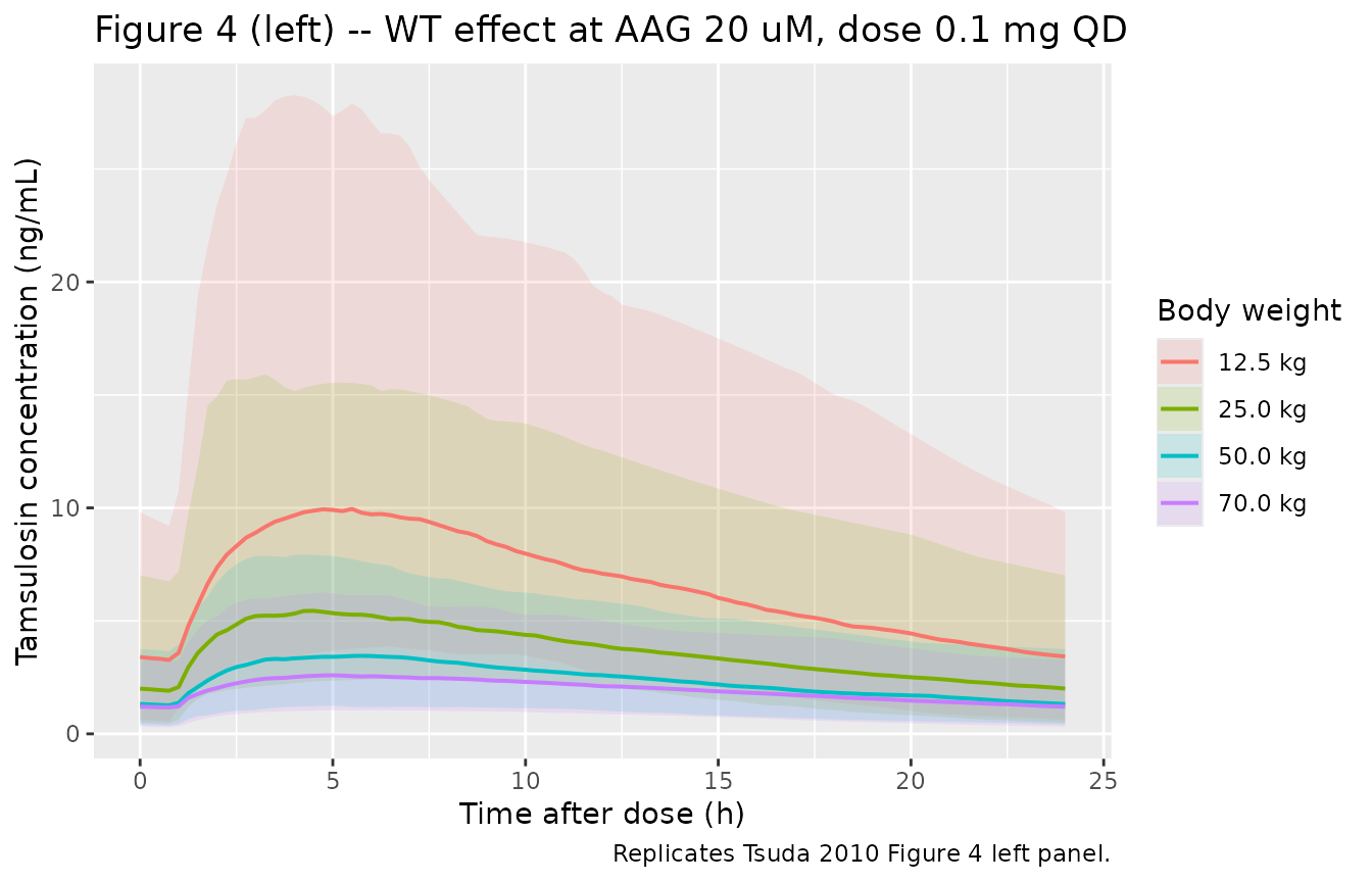
Replicates Tsuda 2010 Figure 4 left panel: median + 5-95 prediction band of plasma tamsulosin concentration after 0.1 mg once daily at steady state (day 10 dosing interval), for four body weights at AAG = 20 uM.
Figure 4 right panel – effect of AAG
Tsuda 2010 Figure 4 right panel shows simulated profiles for four AAG values (10, 20, 30, 40 uM) at the cohort-median WT = 25 kg, dose 0.1 mg. Exposure increases with AAG (negative exponents on both CL/F and V/F).
fig4_aag_window <- sim_fig4_aag |>
  filter(time >= last_dose_time, time <= last_dose_time + 24) |>
  mutate(time_after_dose = time - last_dose_time)

fig4_aag_summary <- fig4_aag_window |>
  group_by(cohort, time_after_dose) |>
  summarise(Q05 = quantile(Cc, 0.05),
            Q50 = quantile(Cc, 0.50),
            Q95 = quantile(Cc, 0.95),
            .groups = "drop")

ggplot(fig4_aag_summary, aes(time_after_dose, Q50, colour = cohort, fill = cohort)) +
  geom_ribbon(aes(ymin = Q05, ymax = Q95), alpha = 0.15, colour = NA) +
  geom_line(linewidth = 0.7) +
  labs(x = "Time after dose (h)",
       y = "Tamsulosin concentration (ng/mL)",
       colour = "AAG (uM)", fill = "AAG (uM)",
       title = "Figure 4 (right) -- AAG effect at WT 25 kg, dose 0.1 mg QD",
       caption = "Replicates Tsuda 2010 Figure 4 right panel.")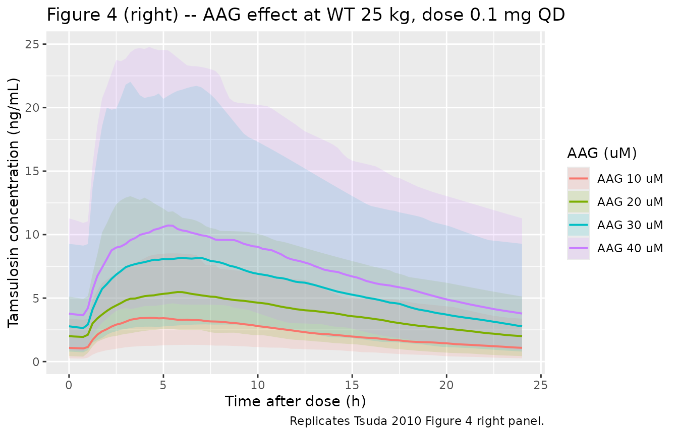
Replicates Tsuda 2010 Figure 4 right panel: median + 5-95 prediction band of plasma tamsulosin concentration after 0.1 mg once daily at steady state for four AAG concentrations at WT = 25 kg.
PKNCA validation
Steady-state NCA over the day-10 dosing interval (tau = 24 h) gives Cmax,ss, Tmax, AUC0-tau, and trough Cmin by body-weight band (Figure 4 left scenario) and by AAG band (Figure 4 right scenario).
nca_wt_window <- sim_fig4_wt |>
  filter(time >= last_dose_time, time <= last_dose_time + 24) |>
  mutate(time_after_dose = time - last_dose_time) |>
  select(id, time = time_after_dose, Cc, cohort)

# Guarantee a time = 0 row per (id, cohort); for extravascular pre-dose Cc = 0
# (steady-state interval starts at the new dose with the pre-dose concentration
# already drained to the trough, so Cc(0) = trough; the bind_rows pattern keeps
# the first row that already exists if there's one, otherwise inserts Cc = 0).
nca_wt_window <- bind_rows(
  nca_wt_window,
  nca_wt_window |> distinct(id, cohort) |> mutate(time = 0, Cc = 0)
) |>
  distinct(id, cohort, time, .keep_all = TRUE) |>
  arrange(id, cohort, time)

dose_wt_df <- fig4_wt |>
  mutate(time = 0, amt = 0.1) |>
  select(id, time, amt, cohort)

conc_obj_wt <- PKNCA::PKNCAconc(nca_wt_window, Cc ~ time | cohort + id,
                                 concu = "ng/mL", timeu = "h")
dose_obj_wt <- PKNCA::PKNCAdose(dose_wt_df, amt ~ time | cohort + id,
                                 doseu = "mg")
intervals_ss <- data.frame(start    = 0,
                           end      = 24,
                           cmax     = TRUE,
                           tmax     = TRUE,
                           auclast  = TRUE,
                           cmin     = TRUE)
nca_res_wt <- suppressMessages(suppressWarnings(
  PKNCA::pk.nca(PKNCA::PKNCAdata(conc_obj_wt, dose_obj_wt, intervals = intervals_ss))
))
nca_aag_window <- sim_fig4_aag |>
  filter(time >= last_dose_time, time <= last_dose_time + 24) |>
  mutate(time_after_dose = time - last_dose_time) |>
  select(id, time = time_after_dose, Cc, cohort)

nca_aag_window <- bind_rows(
  nca_aag_window,
  nca_aag_window |> distinct(id, cohort) |> mutate(time = 0, Cc = 0)
) |>
  distinct(id, cohort, time, .keep_all = TRUE) |>
  arrange(id, cohort, time)

dose_aag_df <- fig4_aag |>
  mutate(time = 0, amt = 0.1) |>
  select(id, time, amt, cohort)

conc_obj_aag <- PKNCA::PKNCAconc(nca_aag_window, Cc ~ time | cohort + id,
                                  concu = "ng/mL", timeu = "h")
dose_obj_aag <- PKNCA::PKNCAdose(dose_aag_df, amt ~ time | cohort + id,
                                  doseu = "mg")
nca_res_aag <- suppressMessages(suppressWarnings(
  PKNCA::pk.nca(PKNCA::PKNCAdata(conc_obj_aag, dose_obj_aag, intervals = intervals_ss))
))
Comparison against published exposure ratios
Tsuda 2010 Results ‘Simulation’ and Discussion paragraph 4 report the exposure-ratio summaries below at steady state with dose 0.1 mg once daily. The published values are exposure ratios (relative to the cohort-median reference within each panel), so the comparison table is built from the simulated AUC0-tau and Cmax,ss medians normalised the same way.
sim_summary_wt <- as.data.frame(nca_res_wt$result) |>
  filter(PPTESTCD %in% c("cmax", "auclast")) |>
  group_by(cohort, PPTESTCD) |>
  summarise(median = median(PPORRES, na.rm = TRUE), .groups = "drop") |>
  tidyr::pivot_wider(names_from = PPTESTCD, values_from = median) |>
  arrange(factor(cohort, levels = c("12.5 kg", "25.0 kg", "50.0 kg", "70.0 kg")))

ratio_wt <- sim_summary_wt |>
  mutate(ratio_cmax_to_70kg = cmax    / cmax[cohort    == "70.0 kg"],
         ratio_auc_to_70kg  = auclast / auclast[cohort == "70.0 kg"])

sim_summary_aag <- as.data.frame(nca_res_aag$result) |>
  filter(PPTESTCD %in% c("cmax", "auclast")) |>
  group_by(cohort, PPTESTCD) |>
  summarise(median = median(PPORRES, na.rm = TRUE), .groups = "drop") |>
  tidyr::pivot_wider(names_from = PPTESTCD, values_from = median) |>
  arrange(factor(cohort, levels = c("AAG 10 uM", "AAG 20 uM", "AAG 30 uM", "AAG 40 uM")))

ratio_aag <- sim_summary_aag |>
  mutate(ratio_cmax_to_10uM = cmax    / cmax[cohort    == "AAG 10 uM"],
         ratio_auc_to_10uM  = auclast / auclast[cohort == "AAG 10 uM"])

# Published values from Tsuda 2010 Results 'Simulation' and Discussion paragraph 4
# Body-weight ratios refer to 12.5 kg patients vs. 70 kg patients at AAG = 20 uM
# AAG ratios refer to AAG 40 uM vs. AAG 10 uM at WT = 25 kg
published <- tibble::tibble(
  Quantity = c("AUC ratio 12.5 kg / 70 kg",
               "Cmax ratio 12.5 kg / 70 kg",
               "AUC ratio AAG 40 / AAG 10",
               "Cmax ratio AAG 40 / AAG 10"),
  Reference = c(3.5, 4.3, 3.2, 3.0),
  Simulated = c(ratio_wt$ratio_auc_to_70kg [ratio_wt$cohort  == "12.5 kg"],
                ratio_wt$ratio_cmax_to_70kg[ratio_wt$cohort  == "12.5 kg"],
                ratio_aag$ratio_auc_to_10uM [ratio_aag$cohort == "AAG 40 uM"],
                ratio_aag$ratio_cmax_to_10uM[ratio_aag$cohort == "AAG 40 uM"])
) |>
  mutate(`% diff` = round(100 * (Simulated - Reference) / Reference, 1),
         flag     = ifelse(abs(`% diff`) > 20, " *", ""))

knitr::kable(
  published |> mutate(Reference = sprintf("%.2f", Reference),
                      Simulated = sprintf("%.2f", Simulated),
                      `% diff` = paste0(sprintf("%.1f", `% diff`), flag)) |>
    select(-flag),
  caption = "Tsuda 2010 Figure 4 / Discussion exposure ratios -- simulated vs. published. * differs from published by > 20%.",
  align = c("l", "r", "r", "r")
)| Quantity | Reference | Simulated | % diff |
|---|---|---|---|
| AUC ratio 12.5 kg / 70 kg | 3.50 | 3.32 | -5.2 |
| Cmax ratio 12.5 kg / 70 kg | 4.30 | 3.94 | -8.5 |
| AUC ratio AAG 40 / AAG 10 | 3.20 | 3.30 | 3.0 |
| Cmax ratio AAG 40 / AAG 10 | 3.00 | 3.02 | 0.5 |
Typical-value steady-state at adult-equivalent weight
The paper reports (Discussion paragraph 5) a typical model-derived half-life of 12 h at a paediatric body weight of 73 kg and a Tmax around 6 h at 70 kg. The typical-value simulation below evaluates both.
# Simulate single-dose 0.1 mg at WT = 73 kg, AAG = 20 uM, characterise lambda_z
demo_73 <- tibble(id = 1L, WT = 73, AAG = 20, cohort = "73 kg typical")
events_73 <- build_events(demo_73, dose_mg = 0.1, n_doses = 10,
                          obs_grid = c(seq(0, 24, by = 0.25),
                                       seq(24.25, 240, by = 0.25)))
sim_73 <- rxode2::rxSolve(mod_typical, events = events_73,
                          keep = c("cohort", "WT", "AAG")) |> as.data.frame()
#> ℹ omega/sigma items treated as zero: 'etalcl', 'etalvc', 'etalka'

# Steady-state day-10 dosing interval
ss_73 <- sim_73 |>
  filter(time >= last_dose_time, time <= last_dose_time + 24) |>
  mutate(time_after_dose = time - last_dose_time)

tmax_73 <- ss_73$time_after_dose[which.max(ss_73$Cc)]
cmax_73 <- max(ss_73$Cc)

# Half-life from the typical-value structural parameters: t1/2 = ln(2) / kel
# = ln(2) * (V/F at WT 73, AAG 20) / (CL/F at WT 73, AAG 20)
vF_73 <- 37.5 * (73 / 70)^1   * (20 / 20)^-0.663
clF_73 <- 2.28 * (73 / 70)^0.75 * (20 / 20)^-0.844
thalf_73 <- log(2) * vF_73 / clF_73

tbl_typical <- tibble::tibble(
  Quantity = c("Tmax at steady state, WT 73 kg, AAG 20 uM (h)",
               "Typical half-life from V/F divided by CL/F at WT 73 kg (h)"),
  Reference = c("~6 h (Tsuda 2010 Discussion paragraph 5; adult Tmax 6-7 h)",
                "12 h (Tsuda 2010 Discussion paragraph 5; adult half-life 13-16 h)"),
  Simulated = c(sprintf("%.2f", tmax_73),
                sprintf("%.2f", thalf_73))
)
knitr::kable(tbl_typical,
             caption = "Typical-value Tmax and half-life at the adult-equivalent paediatric weight of 73 kg.",
align = c("l", "l", "r"))| Quantity | Reference | Simulated |
|---|---|---|
| Tmax at steady state, WT 73 kg, AAG 20 uM (h) | ~6 h (Tsuda 2010 Discussion paragraph 5; adult Tmax 6-7 h) | 6.00 |
| Typical half-life from V/F divided by CL/F at WT 73 kg (h) | 12 h (Tsuda 2010 Discussion paragraph 5; adult half-life 13-16 h) | 11.52 |
Assumptions and deviations
- Allometric exponents fixed at theory values. Tsuda 2010 Results ‘Model building’ Step 2 estimated 0.768 (95% CI 0.598-0.938) for CL/F and 0.807 (95% CI 0.603-1.01) for V/F. Because both CIs include the theory values 0.75 and 1.0, the authors fixed the exponents at those values in the final model (Methods Step 2 paragraph 1). The model file uses the fixed theory values per the published final model.
- IIV variance convention. Tsuda 2010 Table 3 reports IIVs as %CV and a raw between-CL-and-V covariance of 0.238 with an interpreted correlation of 0.715. The simpler %CV = 100 x omega approximation is consistent with the reported covariance and correlation (0.715 x 0.544 x 0.612 = 0.238), so the model file uses omega^2 = (CV / 100)^2 (i.e., 0.2959 / 0.3745 / 1.3689 for CL/F / V/F / ka) rather than the exact log-normal omega^2 = log(1 + CV^2). See the in-file ini() comment block for the verification.
- Inter-occasion variability not separated. Tsuda 2010 reports only IIV and does not partition between-subject from between-occasion variability; the model carries the reported variances as BSV-equivalent.
-
AAG units overridden from g/L to uM. The
canonical-register AAG entry is in g/L (Kloft 2006 / Netterberg 2017
cytotoxic-chemotherapy family); Tsuda 2010 reports AAG in uM with
reference 20 uM, and the published exponents -0.844 (CL/F) and -0.663
(V/F) only apply when AAG enters the model in uM. The model file
overrides
covariateData[[AAG]]$units = "uM". Conversion factor: 1 uM ~ 0.041 g/L assuming the conventional 41 kDa AAG molecular weight (so 20 uM ~ 0.82 g/L). -
Covariates screened but not retained are documented in
covariatesDataExcluded: age, sex, height, BMI, BSA, serum creatinine, creatinine clearance, gamma-glutamyl transferase, haemoglobin, anti- cholinergic concomitant therapy, neurogenic-bladder patient population, and race were all tested and dropped during the Tsuda 2010 stepwise covariate analysis (forward inclusion -> backward elimination). They are recorded as metadata-only so the screening provenance is preserved without producing convention warnings. - Vignette uses 200 subjects per weight or AAG band. This is small enough for the rendered vignette to finish well under the pkgdown 5-minute gate but large enough for stable median exposures. The reported ratios in the comparison table use the simulated cohort medians (the same statistic Tsuda 2010 reports).
-
Bioavailability not parameterised. Tsuda 2010 only
reports apparent parameters CL/F and V/F because no intravenous data
were available. The model file follows the paper and does not include an
lfdepotterm; users who want to separate absolute disposition from F must scale externally. - Modified-release formulation simplified to first-order absorption + lag. The paper’s structural model is a first-order absorption with a lag time (Methods ‘Step 1’; alternative zero-order and sequential zero-then-first- order absorption forms were tested and not selected). The 0.957 h lag-time estimate is consistent with the modified-release capsule sprinkled over applesauce or yogurt.