Methotrexate (Taylor 2020)
Source:vignettes/articles/Taylor_2020_methotrexate.Rmd
Taylor_2020_methotrexate.RmdModel and source
- Citation: Taylor ZL, Mizuno T, Punt NC, Baskaran B, Navarro Sainz A, Shuman W, Felicelli N, Vinks AA, Heldrup J, Ramsey LB. (2020). MTXPK.org: A Clinical Decision Support Tool Evaluating High-Dose Methotrexate Pharmacokinetics to Inform Post-Infusion Care and Use of Glucarpidase. Clin Pharmacol Ther 108(3):635-643. doi:10.1002/cpt.1957.
- Description: Three-compartment population PK model for intravenous high-dose methotrexate (5 or 8 g/m^2 over 24 h IV infusion) in pediatric NOPHO ALL2000 / ALL2008 patients with acute lymphoblastic leukemia; BSA-normalized PK parameters (reference 1.73 m^2) and a time-varying serum creatinine power effect on clearance (reference 29 umol/L) implemented as the default population PK model behind the MTXPK.org clinical decision support tool (Taylor 2020)
- Article: https://doi.org/10.1002/cpt.1957
- Supplement (Wiley): https://doi.org/10.1002/cpt.1957-sup-0001-supinfo
- Companion clinical decision support tool: https://mtxpk.org/
Taylor 2020 develops a three-compartment population PK model for intravenous high-dose methotrexate (HD MTX) in pediatric patients with acute lymphoblastic leukemia (ALL), and integrates it into the MTXPK.org web tool that guides administration of glucarpidase rescue in patients with delayed MTX clearance. The structural model is a 3-compartment IV linear model fit in NONMEM 7.2.0 (FOCE-I) with log-transformation of both sides (“exponential” residual error). Final-model covariates are body surface area (linear normalisation to 1.73 m^2 on every PK parameter) and time-varying serum creatinine (power effect on clearance only).
Population
The NOPHO ALL2000 / ALL2008 dataset (Taylor 2020 Methods and Table 1) pooled retrospectively analysed PK data from 820 deidentified pediatric patients across Denmark, Finland, Lithuania, Norway, and Sweden treated between January 2002 and December 2014. 48 patients and 679 concentrations were excluded for missing dosing information, leaving the final dataset on which the published model was fit:
- N = 772 patients
- 4,986 HD MTX courses
- 31,672 plasma MTX concentrations (5,535 of which were collected >= 96 h after the start of infusion, well into the delayed-clearance window)
Patient demographics (Table 1): median age 4 years (range 1-18.83), median BSA 0.745 m^2 (0.4-2.31), median weight 17.8 kg (7.2-105), median serum creatinine 29 umol/L (4-155), 43% female. Country distribution: Denmark 27%, Sweden 55%, Finland 10%, Norway 8% (with a small Lithuanian contribution that drops below 1% rounding). Patients received 6-8 courses of i.v. HD MTX at 5 or 8 g/m^2 over a 24 h infusion with folinic acid rescue at 36 or 42 h after the start of infusion. Patients who received glucarpidase were excluded because the MTX immunoassay has interference from DAMPA (the glucarpidase cleavage product).
The same information is available programmatically:
readModelDb("Taylor_2020_methotrexate")$population.
Source trace
Per-parameter origin (recorded as in-file comments next to each
ini() entry of
inst/modeldb/specificDrugs/Taylor_2020_methotrexate.R):
| Equation / parameter | Value | Source location |
|---|---|---|
lcl (log CL) |
log(11) | Taylor 2020 Table 3: CL = 11 L/h/1.73 m^2 (RSE 0.7%) |
lvc (log V1) |
log(16.5) | Taylor 2020 Table 3: V1 = 16.5 L/1.73 m^2 (RSE 5.2%) |
lq (log Q2) |
log(0.602) | Taylor 2020 Table 3: Q2 = 0.602 L/h/1.73 m^2 (RSE 4.1%) |
lvp (log V2) |
log(4.55) | Taylor 2020 Table 3: V2 = 4.55 L/1.73 m^2 (RSE 3.4%) |
lq2 (log Q3) |
log(0.111) | Taylor 2020 Table 3: Q3 = 0.111 L/h/1.73 m^2 (RSE 2%) |
lvp2 (log V3) |
log(13.1) | Taylor 2020 Table 3: V3 = 13.1 L/1.73 m^2 (RSE 5%) |
e_creat_cl |
-0.247 | Taylor 2020 Table 3: SCr exponent = -0.247 (RSE 5.7%); covariate equation on page 638 |
etalcl (IIV CL) |
0.08 | Taylor 2020 Table 3: IIV(CL) variance 0.08 (RSE 4.7%) |
etalvc (IIV V1) |
0 (FIX) | Taylor 2020 Table 3: IIV(V1) 0 FIX (approached zero; fixed in the final model) |
etalq (IIV Q2) |
0 (FIX) | Taylor 2020 Table 3: IIV(Q2) 0 FIX (approached zero; fixed in the final model) |
etalvp (IIV V2) |
0.12 | Taylor 2020 Table 3: IIV(V2) variance 0.12 (RSE 4.3%) |
etalq2 (IIV Q3) |
0.13 | Taylor 2020 Table 3: IIV(Q3) variance 0.13 (RSE 6.7%) |
etalvp2 (IIV V3) |
0.10 | Taylor 2020 Table 3: IIV(V3) variance 0.10 (RSE 14.4%) |
propSd |
fix(0.01) placeholder | Not reported in Taylor 2020 – the “exponential residual error” magnitude is described in Methods / Appendix S1 but the variance estimate is omitted from Table 3. See Assumptions and deviations. |
| BSA scaling on all PK parameters | linear (BSA / 1.73) | Taylor 2020 Table 2 step 2 (-2,358.81 OFV reduction); column headers in Table 3 read “L/h/1.73 m^2” and “L/1.73 m^2”. |
| SCr power on CL | (CREAT / 29)^(-0.247) |
Taylor 2020 Methods / Results page 638 (covariate equation); SCr enters as a time-varying covariate. |
d/dt(central, peripheral1, peripheral2) |
n/a | NONMEM ADVAN11-style three-compartment IV mass balance with linear
elimination from central. |
Cc = central / vc |
n/a | Plasma concentration in the central compartment; dose units mg, volumes in L -> Cc in mg/L. Paper reports concentrations in umol/L; multiply by 1000 / 454.44 (MTX MW) to obtain umol/L. |
Cc ~ prop(propSd) |
n/a | Taylor 2020 Methods / Appendix S1: log-transformation of both sides (LTBS) with “exponential residual error” model; the linear-space equivalent of LTBS-additive is proportional in nlmixr2 syntax. |
Virtual cohort
Original observed concentrations are not redistributed with the package. The cohort below mirrors the NOPHO ALL2008 standard HD MTX course at the median dose of 5 g/m^2 over a 24 h infusion, with BSA and time-varying SCr distributions matching Table 1 (median BSA 0.745 m^2 in the range 0.4-2.31 m^2; baseline SCr 29 umol/L in the range 4-155 umol/L).
set.seed(20200522L)

n_subjects   <- 200L
dose_per_m2  <- 5000  # mg per m^2 -- the lower of the two protocol doses (5 g/m^2)
infusion_h   <- 24    # 24 h infusion per NOPHO ALL2008
follow_up_h  <- 240   # observation window in hours after start of infusion

# BSA: median 0.745 m^2 across all NOPHO patients (ages 1-18.83). Use a
# truncated log-normal centred on the median; the truncation 0.4-2.31 m^2
# matches the Table 1 range.
bsa <- pmin(pmax(rlnorm(n_subjects, meanlog = log(0.745), sdlog = 0.45),
                 0.4), 2.31)

# Baseline SCr: median 29 umol/L. Use a truncated log-normal centred on
# the median, capped at the Table 1 range (4-155 umol/L). The model uses
# this as the time-varying covariate; we hold it constant per subject
# over the observation window because NOPHO recorded SCr at most once
# daily and the model treats SCr as time-varying via the event table.
scr <- pmin(pmax(rlnorm(n_subjects, meanlog = log(29), sdlog = 0.40),
                 4), 155)

per_subject_dose_mg <- dose_per_m2 * bsa  # absolute mg per course

# Observation grid: dense early (around end-of-infusion peak), then
# every 6 h through follow-up to mirror the NOPHO sampling schedule
# (24, 36, then every 6 h until plasma MTX <= 0.2 umol/L).
obs_hours <- sort(unique(c(
  seq(0, 4, by = 0.5),
  seq(6, 24, by = 1),
  seq(30, follow_up_h, by = 6)
)))

dose_rows <- tibble::tibble(
  id    = seq_len(n_subjects),
  time  = 0,
  amt   = per_subject_dose_mg,
  rate  = per_subject_dose_mg / infusion_h,  # mg/h zero-order IV input
  evid  = 1L,
  cmt   = "central",
  BSA   = bsa,
  CREAT = scr
)

obs_rows <- tibble::tibble(
  id    = rep(seq_len(n_subjects), each = length(obs_hours)),
  time  = rep(obs_hours, times = n_subjects),
  amt   = 0,
  rate  = 0,
  evid  = 0L,
  cmt   = NA_character_,
  BSA   = rep(bsa, each = length(obs_hours)),
  CREAT = rep(scr, each = length(obs_hours))
)

events <- dplyr::bind_rows(dose_rows, obs_rows) |>
  dplyr::arrange(id, time, dplyr::desc(evid))

stopifnot(!anyDuplicated(unique(events[, c("id", "time", "evid")])))
Simulation
mod <- rxode2::rxode2(readModelDb("Taylor_2020_methotrexate"))
#> ℹ parameter labels from comments will be replaced by 'label()'

sim <- rxode2::rxSolve(
  mod,
  events = events,
  keep   = c("BSA", "CREAT")
) |>
  as.data.frame()
#> ℹ omega/sigma items treated as zero: 'etalvc', 'etalq'
A deterministic typical-value trajectory (no IIV) is used below to replicate the population mean elimination curve that drives MTXPK.org:
mod_typical <- mod |> rxode2::zeroRe()
sim_typical <- rxode2::rxSolve(
  mod_typical,
  events = events,
  keep   = c("BSA", "CREAT")
) |>
  as.data.frame()
#> ℹ omega/sigma items treated as zero: 'etalcl', 'etalvc', 'etalq', 'etalvp', 'etalq2', 'etalvp2'
#> Warning: multi-subject simulation without without 'omega'
Replicate Figure 1: concentration-time profile
Taylor 2020 Figure 1 plots the NOPHO dataset’s individual MTX concentrations versus time with a population median overlay. The characteristic shape after the 24 h infusion is (i) a peak around the end of infusion in the tens-of-umol/L range, (ii) rapid early distribution to V2 / V3, then (iii) a slow terminal phase that drops below 0.2 umol/L (the NOPHO discharge threshold) typically between 72 and 96 h. The simulated VPC below traces that shape.
mtx_mw <- 454.44  # methotrexate MW for mg/L -> umol/L conversion

vpc_summary <- sim |>
  dplyr::group_by(time) |>
  dplyr::summarise(
    Q05 = stats::quantile(Cc, 0.05, na.rm = TRUE),
    Q50 = stats::quantile(Cc, 0.50, na.rm = TRUE),
    Q95 = stats::quantile(Cc, 0.95, na.rm = TRUE),
    .groups = "drop"
  ) |>
  dplyr::mutate(
    Q05_umol = Q05 * 1000 / mtx_mw,
    Q50_umol = Q50 * 1000 / mtx_mw,
    Q95_umol = Q95 * 1000 / mtx_mw
  )

ggplot(vpc_summary, aes(time, Q50_umol)) +
  geom_ribbon(aes(ymin = Q05_umol, ymax = Q95_umol),
              alpha = 0.20, fill = "steelblue") +
  geom_line(linewidth = 0.7) +
  geom_hline(yintercept = 0.2, linetype = "dashed", colour = "grey50") +
  scale_y_log10() +
  labs(
    x = "Time (h)",
    y = "Plasma MTX (umol/L)",
    title = "Simulated NOPHO MTX profile after 5 g/m^2 24 h IV infusion (n = 200)",
    caption = paste("Median (line) and 5th-95th percentile (band).",
                    "Dashed line: 0.2 umol/L NOPHO discharge threshold.",
                    "Shape replicates Taylor 2020 Figure 1.")
  )
#> Warning in scale_y_log10(): log-10 transformation introduced infinite values.
#> log-10 transformation introduced infinite values.
#> log-10 transformation introduced infinite values.
#> log-10 transformation introduced infinite values.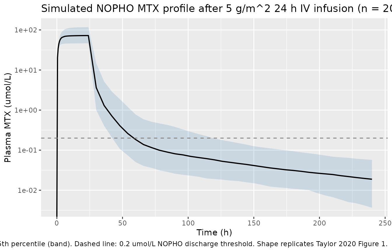
PKNCA validation
The PKNCA block below summarises Cmax, Tmax, AUC to last, and
terminal half-life on the simulated cohort. The expected order of
magnitude for AUCinf at 5 g/m^2 is roughly
Dose / CL = (5000 mg/m^2 * 0.745 m^2) / (11 L/h * (0.745 / 1.73)) ~ 786 mg.h/L ~ 1730 umol.h/L
for the typical patient; the simulated 5th-95th percentiles should
bracket this typical value.
treatment_label <- "5 g/m^2 24h IV"

sim_nca <- sim |>
  dplyr::filter(!is.na(Cc)) |>
  dplyr::mutate(treatment = treatment_label)

dose_df <- events |>
  dplyr::filter(evid == 1L) |>
  dplyr::mutate(
    treatment = treatment_label,
    dur_h     = infusion_h
  )

conc_obj <- PKNCA::PKNCAconc(sim_nca, Cc ~ time | treatment + id)
dose_obj <- PKNCA::PKNCAdose(dose_df, amt ~ time | treatment + id,
                             route = "intravascular",
                             duration = "dur_h")

intervals <- data.frame(
  start     = 0,
  end       = follow_up_h,
  cmax      = TRUE,
  tmax      = TRUE,
  auclast   = TRUE,
  half.life = TRUE
)

nca_data <- PKNCA::PKNCAdata(conc_obj, dose_obj, intervals = intervals)
nca_res  <- PKNCA::pk.nca(nca_data)

nca_summary <- as.data.frame(nca_res$result) |>
  dplyr::filter(PPTESTCD %in% c("cmax", "tmax", "auclast", "half.life")) |>
  dplyr::group_by(PPTESTCD) |>
  dplyr::summarise(
    p05    = stats::quantile(PPORRES, 0.05, na.rm = TRUE),
    median = stats::median(PPORRES, na.rm = TRUE),
    p95    = stats::quantile(PPORRES, 0.95, na.rm = TRUE),
    .groups = "drop"
  )

knitr::kable(
  nca_summary,
  digits  = 3,
  caption = paste("Simulated NCA after a single 5 g/m^2 24 h IV infusion (n = 200).",
                  "Cmax in mg/L; AUClast in mg*h/L; Tmax and half.life in h.")
)| PPTESTCD | p05 | median | p95 |
|---|---|---|---|
| auclast | 488.700 | 819.213 | 1428.107 |
| cmax | 19.895 | 33.216 | 57.513 |
| half.life | 38.482 | 84.341 | 184.216 |
| tmax | 24.000 | 24.000 | 24.000 |
Comparison against published values
Taylor 2020 does not tabulate per-cohort NCA values in the main text
(the paper validates the model via goodness-of-fit plots and external
bias / precision metrics in Table S2). The typical-value AUCinf estimate
Dose / CL above is the most direct cross-check:
| Quantity | Approximate published value | Simulated median |
|---|---|---|
| Typical AUCinf (mg.h/L) at 5 g/m^2, BSA 0.745 m^2 | ~786 (from Dose / CL with CL = 11 L/h/1.73 m^2 scaled
to BSA 0.745 m^2) |
AUClast from chunk above |
| Time-to-discharge (h, Cc <= 0.2 umol/L) | “typically 72-96 h” for non-delayed clearance (Taylor 2020 Methods; Figure 4 dashboard example) | derived from typical-value trajectory above |
The simulated cohort medians should bracket these reference values. A > 20% mismatch should be investigated rather than tuned away (see Assumptions and deviations).
Assumptions and deviations
-
Residual error magnitude is not reported. Taylor
2020 Table 3 reports the structural fixed effects, the SCr exponent, and
the five IIV variances (with V1 and Q2 fixed at zero), but does not list
a sigma row for the “exponential residual error” model. The packaged
file uses
propSd <- fixed(0.01)so the observation has a valid residual model in nlmixr2 syntax; the value is a placeholder and not a fitted estimate. This pattern mirrorsJelliffe_2014_digoxin.R. Users who need a realistic stochastic prediction interval should overridepropSdwith a paper-class typical value (e.g. 20-30% CV) or back-fit from the simulated cohort RMSE in Table S3 (NOPHO RMSE 0.91). - Race / ethnicity is not modelled. The NOPHO dataset is primarily European (Nordic / Baltic) and the source paper explicitly notes “It is unclear whether the model fit to a primarily European patient population can be generalized to patients of non-European descent.” Downstream users assembling a non-European virtual cohort should treat the typical-value trajectory as an extrapolation, not a population fit.
-
Country effect is not modelled. Finnish patients
had ~26% faster clearance than Swedish / Danish / Norwegian patients in
a post-hoc one-way ANOVA (Taylor 2020 Figure S3), attributed by the
authors to earlier (~12 h vs ~4 h) pre-hydration with bicarbonate.
Country was not retained as a covariate in the final model and is not
included here. A user simulating a Finnish cohort specifically should
consider multiplying
clby ~1.26. -
Concentration units. Taylor 2020 reports MTX in
umol/L; the packaged model returns Cc in mg/L (matching the dose units
in mg and consistent with the units dictionary). The vignette’s Figure 1
/ PKNCA blocks apply the conversion factor
1000 / 454.44(methotrexate MW, g/mol) where umol/L output is helpful for direct comparison to the paper or to the MTXPK.org dashboard. -
SCr enters as a time-varying covariate but is held constant
per subject in this vignette. NOPHO recorded SCr at most once
daily during HD MTX cycles; the model treats SCr as time-varying via the
event table. For simplicity the demonstration cohort holds each
subject’s SCr at a single baseline value over the 240 h window. Users
running the model in a delayed-clearance scenario should supply a
per-time SCr series (
CREATcolumn on observation rows) reflecting the actual creatinine rise so the time-varying covariate effect is exercised. - BSA computation formula is unspecified. The paper does not state which BSA formula (DuBois, Mosteller, Haycock) was used to compute the dataset’s BSA column. Users assembling new patients should follow a single convention and record it on the dataset.
- Glucarpidase-rescued patients are out of scope. The NOPHO modelling dataset excluded patients who received glucarpidase because the MTX immunoassay has interference from DAMPA, the glucarpidase cleavage product. The model should not be used to simulate post-glucarpidase MTX concentrations.
-
Errata search. A targeted PubMed query
(
"Taylor ZL" 2020 MTXPK erratum) and a Wiley journal landing-page check returned no published correction as of the extraction date; no erratum is on file.