SGLT2-inhibitor HbA1c dose-response, UGE-normalized (Sato 2024)
Source:vignettes/articles/Sato_2024_sglt2_hba1c_mbma.Rmd
Sato_2024_sglt2_hba1c_mbma.RmdModel and source
Citation: Sato H, Ishikawa A, Yoshioka H, Jin R, Sano Y, Hisaka A. Model-based meta-analysis of HbA1c reduction across SGLT2 inhibitors using dose adjusted by urinary glucose excretion. Sci Rep. 2024 Oct 21;14(1):24695. doi:10.1038/s41598-024-76256-6.
Supplement (analysis code, study tables, dataset): https://doi.org/10.1038/s41598-024-76256-6 (Supplementary Information; MOESM1 R script, MOESM2 search terms and references, MOESM3 Tables S1-S3)
Description: MBMA. Unified class-level dose-response model-based meta-analysis of HbA1c reduction across six sodium-glucose co-transporter-2 (SGLT2) inhibitors – canagliflozin, dapagliflozin, empagliflozin, ipragliflozin, luseogliflozin and tofogliflozin – in type 2 diabetes. The paper’s central device is a UGE-NORMALIZED DOSE: each drug’s mg dose is divided by a drug-specific ‘reference dose’, defined as the dose producing 51.4 g/day of urinary glucose excretion (UGE) in healthy phase I volunteers, which is the geometric mean of the six drugs’ UGE at their clinical doses. After that normalization a SINGLE sigmoid Emax curve describes all six drugs. Emax carries five covariates (baseline HbA1c, body weight, eGFR, drug-naive status and diabetes duration) plus a canagliflozin-specific 1.33-fold potentiation, which the authors attribute to canagliflozin’s comparatively weak SGLT2-over-SGLT1 selectivity; the placebo term carries a concomitant-antihyperglycemic -medication effect. Fitted to 295 study-arm means from 83 published phase II/III randomized trials of at least 12 weeks. The model is purely ALGEBRAIC and time-independent – it predicts the end-of-treatment study-arm mean HbA1c change from baseline, has no ODE states and consumes no rxode2 dose events. Variability is BETWEEN-STUDY (inter-study, ISV), encoded as correlated study-level etas, so the model simulates study-arm mean outcomes and is NOT suitable for individual-subject simulation. Companion SGLT2-inhibitor MBMA on the same endpoint: modellib(‘Yao_2023_sglt2_endpoints_mbma’), which instead drives HbA1c through exposure (AUC) and an FPG turnover model.
Sato 2024 asks whether the six sodium-glucose co-transporter-2 (SGLT2) inhibitors marketed for type 2 diabetes share one dose-response relationship once their doses are put on a common scale. The common scale is urinary glucose excretion (UGE): each drug’s mg dose is divided by the dose that produces 51.4 g/day of UGE in healthy phase I volunteers. After that normalization a single sigmoid Emax curve describes HbA1c reduction across all six drugs, with canagliflozin the one exception – it retains a 1.33-fold larger Emax.
This is a model-based meta-analysis (MBMA). The unit of observation is a published study-arm mean, not a patient. The model is purely algebraic: it predicts the end-of-treatment arm-mean HbA1c change from baseline and has no ODE states, no time course and no dose events.
Population
| Field | Value |
|---|---|
| species | human |
| n_studies | 83 |
| n_data_points | 295 |
| age_range | per-arm mean age approximately 51-66 years (Sato 2024 Supplementary Table S2) |
| weight_range | per-arm mean body weight 61.0-96.7 kg (Sato 2024 Table 2B covariate range) |
| disease_state | Type 2 diabetes mellitus. Per-arm mean baseline HbA1c 7.2-9.1% (NGSP), per-arm mean eGFR 38.5-154.5 mL/min/1.73 m^2 (so the pool spans normal renal function through moderate-to-severe impairment, including dedicated renal-impairment trials), per-arm mean diabetes duration 0.25-18.2 years. Treatment history across the 295 arms: 51 drug-naive, 53 previously treated but on monotherapy in the trial, 191 add-on to background antihyperglycemic therapy. |
| dose_range | Placebo plus canagliflozin 50-300, dapagliflozin 1-50, empagliflozin 1-50, ipragliflozin 12.5-300, luseogliflozin 0.5-10 and tofogliflozin 2.5-40 mg/day; equivalently UGE-normalized doses of roughly 0.07-3.1. Treatment durations 12-104 weeks. |
| regions | International. Canagliflozin, dapagliflozin and empagliflozin trials were mostly conducted outside Japan; ipragliflozin, luseogliflozin and tofogliflozin trials were mostly Japanese (Sato 2024 Supplementary Table S2). |
| notes | Model-based meta-analysis: the unit of observation is a published study-arm mean HbA1c change from baseline, not an individual measurement. 83 trials contributed 295 arms after a PubMed search of phase II/III trials of at least 12 weeks reporting HbA1c (137 studies screened). Per-drug study counts: canagliflozin 17, dapagliflozin 29, empagliflozin 22, ipragliflozin 7, luseogliflozin 5, tofogliflozin 3. The dose-normalization layer is calibrated on a SEPARATE population – healthy Japanese volunteers in six single-dose phase I UGE studies (n = 32-57 per study, mean age 23-27 years, mean body weight 61-65 kg; Sato 2024 Supplementary Table S1) – so the reference doses carry the assumption, defended at length in the paper’s Discussion, that the dose-UGE relationship ranks the six drugs the same way in healthy volunteers as in patients. |
The estimation dataset is 295 study arms from 83 published phase II/III trials of at least 12 weeks that reported HbA1c, identified by a PubMed search of trials to October 2017 (137 screened; Sato 2024 Figure 2 and Supplementary Table S2). Per-drug study counts are canagliflozin 17, dapagliflozin 29, empagliflozin 22, ipragliflozin 7, luseogliflozin 5 and tofogliflozin 3.
The dose-normalization layer is calibrated on a different population: six single-dose phase I UGE studies in healthy Japanese volunteers (n = 32-57 per study, mean age 23-27 years, mean body weight 61-65 kg; Sato 2024 Supplementary Table S1). The paper devotes a Discussion section to defending the transfer, arguing that although the dose-UGE relationship genuinely differs between healthy people and patients, the relative ranking of the six drugs is preserved because all six are at least 100-fold SGLT2-selective and circulate well below their SGLT1 Ki at clinical doses.
Source trace
Every ini() entry carries an in-file comment naming its
source location; the table below collects them.
| Equation / parameter | Value | Source location |
|---|---|---|
| Sigmoid Emax structure | n/a | Sato 2024 Eq. 6 |
Base = theta1 + sum f(COV) + eta1 |
n/a | Sato 2024 Eq. 7 (additive covariates, additive eta) |
Emax = theta2 * prod f(COV) * exp(eta2) |
n/a | Sato 2024 Eq. 8 (multiplicative covariates, exponential eta) |
ED50 = theta3, n = theta4
|
n/a | Sato 2024 Eq. 9-10 (no covariates, no ISV) |
Dose normalization nDose = Dose / Dose_ref
|
n/a | Sato 2024 Eq. 1-5 |
pmax (Base) |
-0.124 | Table 2A; SE 0.0261 (Table S3A) |
emax |
-0.796 | Table 2A; SE 0.071 (Table S3A) |
led50 |
log(0.251) | Table 2A; SE 0.0539 (Table S3A) |
lhill |
log(0.662) | Table 2A; SE 0.149 (Table S3A) |
e_hba1c_emax |
0.438 | Table 2B exp(0.438 (COV - 8)); SE 0.0719 |
e_wt_emax |
-0.661 | Table 2B (COV/81.6)^-0.661; SE 0.175 |
e_cana_emax |
0.328 | Table 2B “Cana: 1.33”; theta from Table S3A, SE 0.045 |
e_crcl_emax |
0.821 | Table 2B (COV/85.9)^0.821; SE 0.102 |
e_trt_t2dm_naive_emax |
0.230 | Table 2B “No: 1.230”; SE 0.081 |
e_t_diag_diab_emax |
-0.025 | Table 2B 1 - 0.025 (COV - 6.6); SE 0.0077 |
e_trt_t2dm_addon_pmax |
0.156 | Table 2B “No: 0.156”; SE 0.0348 |
| ISV omegas + correlation | 0.191, 0.214, 0.785 | Table 2A “ISV (omega)” column |
Residual sigma
|
fixed 1 | Sato 2024 Eq. 6 text |
dref_* (six reference doses) |
see below | Figure 1, digitized – not printed anywhere |
The UGE dose-normalization layer
Sato 2024 fits a linear-logarithmic dose-UGE curve per drug (Eq. 1,
UGE = a + b*log10(Dose)), takes the geometric mean of the
six drugs’ UGE at their clinical doses as the reference
UGE (51.4 g/day, Eq. 2-3), and inverts each drug’s curve at
that value to get its reference dose (Eq. 4).
The six reference doses are the only quantities in this extraction
that the paper never prints: they appear solely as the red dashed
vertical lines in Figure 1, and the underlying data_uge.csv
read by the authors’ analysis script is not distributed. They were
recovered by digitizing Figure 1 at 600 dpi and cross-checked two
independent ways (see Assumptions and deviations).
| Drug | Reference dose (mg/day) | Curve-fit cross-check | Clinical dose (mg/day) | Agreement (%) |
|---|---|---|---|---|
| Canagliflozin | 97.70 | 96.69 | 100 | 1.03 |
| Dapagliflozin | 7.05 | 7.02 | 5, 10 | 0.43 |
| Empagliflozin | 11.80 | 11.90 | 10, 25 | 0.85 |
| Ipragliflozin | 79.00 | 80.33 | 50, 100 | 1.68 |
| Luseogliflozin | 7.38 | 7.38 | 2.5, 5 | 0.00 |
| Tofogliflozin | 15.00 | 14.59 | 20 | 2.73 |
The two routes agree to within 1.7% on every drug, and the log-linear form of Eq. 1 is confirmed by the curve extraction at R-squared 0.982-0.999. The x-axis calibration itself was validated by locating the clinical-dose markers via their exact palette colours from the authors’ script: the recovered positions reproduce the known clinical doses (100, 10, 100, 5 and 20 mg) to within 0.1-1%.
Setting up simulations
The model consumes six per-arm daily-dose covariate columns plus five
patient covariates. There are no dose events and no time course, so an
“event table” here is one row per study arm at
time = 0.
mod  <- readModelDb("Sato_2024_sglt2_hba1c_mbma")
# Typical-value (population) predictions: zero the between-study etas AND the
# residual. The residual sigma is fixed at 1 on a STANDARDIZED scale (see the
# Assumptions section), so leaving it in would add a nonsensical 1-point SD.
tv <- rxode2::zeroRe(mod)

dose_cols <- c("DOSE_CANA_MGD", "DOSE_DAPA_MGD", "DOSE_EMPA_MGD",
               "DOSE_IPRA_MGD", "DOSE_LUSEO_MGD", "DOSE_TOFO_MGD")

# Reference arm: every covariate at the centering value used by Sato 2024, so
# every f(COV) equals exactly 1. Background antihyperglycemic therapy present
# (TRT_T2DM_ADDON = 1) so the placebo covariate contributes 0 as well.
ref_arm <- function(n = 1L) {
  out <- data.frame(
    id = seq_len(n), time = 0,
    HBA1C = 8, WT = 81.6, CRCL = 85.9, T_DIAG_DIAB = 6.6,
    TRT_T2DM_NAIVE = 0, TRT_T2DM_ADDON = 1
  )
  for (cc in dose_cols) out[[cc]] <- 0
  out
}

# Solve a set of arms and return the input frame with model outputs attached.
# rxSolve drops the `id` column for a single subject (known rxode2 behaviour),
# so guard rather than assume.
solve_arms <- function(arms, model = tv) {
  s <- rxode2::rxSolve(model, arms, returnType = "data.frame")
  if (is.null(s$id)) s$id <- 1L
  stopifnot(nrow(s) == nrow(arms), !anyDuplicated(s$id))
  idx <- match(arms$id, s$id)
  stopifnot(!anyNA(idx))
  arms$ndose   <- s$ndose[idx]
  arms$base    <- s$base[idx]
  arms$emaxArm <- s$emaxArm[idx]
  arms$Cc      <- s$Cc[idx]
  arms
}
Validation 1: the paper’s printed anchor point
Sato 2024 Results states outright: “The estimated HbA1c change at
the normalized dose = 1.0 was -0.692%.” That single printed number
is a closed-form test of Base, Emax,
ED50 and n together, and of the sigmoid Emax
structure. Because it is a typical-value, deterministic
quantity – not a statistic of a simulated cohort – it is asserted to
full printed precision.
anchor <- ref_arm()
anchor$DOSE_EMPA_MGD <- 11.8            # exactly one reference dose of empagliflozin
anchor <- solve_arms(anchor)
#> ℹ omega/sigma items treated as zero: 'eta_study_pmax', 'eta_study_emax'

# Independent hand-evaluation of Sato 2024 Eq. 6 at nDose = 1.
closed_form <- -0.124 + -0.796 * 1^0.662 / (0.251^0.662 + 1^0.662)

tibble::tibble(
  Quantity  = c("Normalized dose", "Model Cc", "Closed form (Eq. 6 by hand)", "Sato 2024 printed value"),
  Value     = c(anchor$ndose, anchor$Cc, closed_form, -0.692)
) |>
knitr::kable(digits = 5, caption = "Sato 2024 printed anchor: HbA1c change at normalized dose 1.0.")| Quantity | Value |
|---|---|
| Normalized dose | 1.00000 |
| Model Cc | -0.69238 |
| Closed form (Eq. 6 by hand) | -0.69238 |
| Sato 2024 printed value | -0.69200 |
Validation 2: the placebo term
Base is the placebo-arm HbA1c change and carries the
only additive covariate (Table 2B: concomitant medications “Yes: 0; No:
0.156”). Both levels are printed, so both are checked.
pbo <- ref_arm(2L)
pbo$TRT_T2DM_ADDON <- c(1, 0)           # with / without background therapy
pbo <- solve_arms(pbo)
#> ℹ omega/sigma items treated as zero: 'eta_study_pmax', 'eta_study_emax'
#> Warning: multi-subject simulation without without 'omega'

tibble::tibble(
  Arm      = c("Placebo, on background therapy", "Placebo, no background therapy"),
  Model    = pbo$Cc,
  Expected = c(-0.124, -0.124 + 0.156)
) |>
knitr::kable(digits = 4, caption = "Placebo-arm HbA1c change (Sato 2024 Table 2A Base, Table 2B concomitant-medication effect).")| Arm | Model | Expected |
|---|---|---|
| Placebo, on background therapy | -0.124 | -0.124 |
| Placebo, no background therapy | 0.032 | 0.032 |
An arm with no background therapy is predicted to rise by
0.032 points under placebo, while an add-on arm falls by 0.124 – the
same direction of effect the sibling SGLT2 MBMA
modellib("Yao_2023_sglt2_endpoints_mbma") finds, where
placebo FPG rises in every treatment-history stratum except add-on.
Validation 3: every covariate range in Table 2B
Table 2B prints, for each covariate, the observed covariate range
and the corresponding range of f(COV).
That is 12 printed numbers across 6 continuous and categorical effects,
and it is an enumerating check – the table below is generated
by iterating the covariate list, so a covariate added to the model
without a matching row here would show up as a missing entry rather than
pass silently.
# One row per printed Table 2B covariate: the covariate column, the endpoints
# of the printed COVrange, and the printed f(COV) values at those endpoints.
cov_spec <- tibble::tribble(
  ~label,                       ~column,          ~lo,   ~hi,    ~f_lo,  ~f_hi,
  "Baseline HbA1c [%]",         "HBA1C",           7.2,   9.1,    0.704,  1.62,
  "Body weight [kg]",           "WT",             61.0,  96.7,    1.21,   0.894,
  "GFR [mL/min/1.73 m2]",       "CRCL",           38.5, 154.5,    0.517,  1.62,
  "Diabetic duration [years]",  "T_DIAG_DIAB",     0.25, 18.2,    1.16,   0.71,
  "Pre-treatment (naive)",      "TRT_T2DM_NAIVE",  0,     1,      1,      1.230,
  "Canagliflozin",              "DOSE_CANA_MGD",   0,    97.7,    1,      1.33
)

# f(COV) is recovered as the ratio of the arm's Emax to the reference Emax.
emax_ref <- solve_arms(ref_arm())$emaxArm
#> ℹ omega/sigma items treated as zero: 'eta_study_pmax', 'eta_study_emax'

f_at <- function(column, value) {
  a <- ref_arm()
  a[[column]] <- value
  # A canagliflozin dose would also change nDose, but f(COV) is read off Emax,
  # which is independent of dose -- so this isolates the covariate cleanly.
  solve_arms(a)$emaxArm / emax_ref
}

cov_check <- cov_spec |>
  rowwise() |>
  mutate(model_lo = f_at(column, lo), model_hi = f_at(column, hi)) |>
  ungroup() |>
  mutate(worst_abs_diff = pmax(abs(model_lo - f_lo), abs(model_hi - f_hi)))
#> ℹ omega/sigma items treated as zero: 'eta_study_pmax', 'eta_study_emax'
#> ℹ omega/sigma items treated as zero: 'eta_study_pmax', 'eta_study_emax'
#> ℹ omega/sigma items treated as zero: 'eta_study_pmax', 'eta_study_emax'
#> ℹ omega/sigma items treated as zero: 'eta_study_pmax', 'eta_study_emax'
#> ℹ omega/sigma items treated as zero: 'eta_study_pmax', 'eta_study_emax'
#> ℹ omega/sigma items treated as zero: 'eta_study_pmax', 'eta_study_emax'
#> ℹ omega/sigma items treated as zero: 'eta_study_pmax', 'eta_study_emax'
#> ℹ omega/sigma items treated as zero: 'eta_study_pmax', 'eta_study_emax'
#> ℹ omega/sigma items treated as zero: 'eta_study_pmax', 'eta_study_emax'
#> ℹ omega/sigma items treated as zero: 'eta_study_pmax', 'eta_study_emax'
#> ℹ omega/sigma items treated as zero: 'eta_study_pmax', 'eta_study_emax'
#> ℹ omega/sigma items treated as zero: 'eta_study_pmax', 'eta_study_emax'

cov_check |>
  select(label, lo, hi, f_lo, model_lo, f_hi, model_hi, worst_abs_diff) |>
  rename(
    "Covariate"        = label,
    "COV low"          = lo,
    "COV high"         = hi,
    "f(COV) printed @low"  = f_lo,
    "f(COV) model @low"    = model_lo,
    "f(COV) printed @high" = f_hi,
    "f(COV) model @high"   = model_hi,
    "Worst abs. diff"      = worst_abs_diff
  ) |>
knitr::kable(digits = 4, caption = "Every covariate effect range printed in Sato 2024 Table 2B, reproduced from the packaged model.")| Covariate | COV low | COV high | f(COV) printed @low | f(COV) model @low | f(COV) printed @high | f(COV) model @high | Worst abs. diff |
|---|---|---|---|---|---|---|---|
| Baseline HbA1c [%] | 7.20 | 9.1 | 0.704 | 0.7044 | 1.620 | 1.6190 | 0.0010 |
| Body weight [kg] | 61.00 | 96.7 | 1.210 | 1.2121 | 0.894 | 0.8938 | 0.0021 |
| GFR [mL/min/1.73 m2] | 38.50 | 154.5 | 0.517 | 0.5174 | 1.620 | 1.6192 | 0.0008 |
| Diabetic duration [years] | 0.25 | 18.2 | 1.160 | 1.1587 | 0.710 | 0.7100 | 0.0012 |
| Pre-treatment (naive) | 0.00 | 1.0 | 1.000 | 1.0000 | 1.230 | 1.2300 | 0.0000 |
| Canagliflozin | 0.00 | 97.7 | 1.000 | 1.0000 | 1.330 | 1.3280 | 0.0020 |
Validation 4: the six drugs collapse onto one curve
The paper’s central claim is that after UGE normalization the six drugs share a dose-response. Dosing each drug at exactly its own reference dose must therefore give an identical prediction – except canagliflozin, which is 1.33-fold more potent (Sato 2024 Figure 5).
dref <- c(DOSE_CANA_MGD = 97.7, DOSE_DAPA_MGD = 7.05, DOSE_EMPA_MGD = 11.8,
          DOSE_IPRA_MGD = 79.0, DOSE_LUSEO_MGD = 7.38, DOSE_TOFO_MGD = 15.0)

uni <- ref_arm(length(dref))
for (i in seq_along(dref)) uni[i, names(dref)[i]] <- dref[[i]]
uni$Drug <- c("Canagliflozin", "Dapagliflozin", "Empagliflozin",
              "Ipragliflozin", "Luseogliflozin", "Tofogliflozin")
uni <- solve_arms(uni)
#> ℹ omega/sigma items treated as zero: 'eta_study_pmax', 'eta_study_emax'
#> Warning: multi-subject simulation without without 'omega'

uni |>
  select(Drug, ndose, Cc) |>
  rename("Normalized dose" = ndose, "HbA1c change (%)" = Cc) |>
knitr::kable(digits = 4, caption = "Each drug dosed at its own UGE reference dose (normalized dose = 1).")| Drug | Normalized dose | HbA1c change (%) |
|---|---|---|
| Canagliflozin | 1 | -0.8788 |
| Dapagliflozin | 1 | -0.6924 |
| Empagliflozin | 1 | -0.6924 |
| Ipragliflozin | 1 | -0.6924 |
| Luseogliflozin | 1 | -0.6924 |
| Tofogliflozin | 1 | -0.6924 |
others <- uni$Cc[uni$Drug != "Canagliflozin"]
cana   <- uni$Cc[uni$Drug == "Canagliflozin"]
stopifnot(
  all(abs(uni$ndose - 1) < 1e-8),          # reference doses are self-consistent
  diff(range(others)) < 1e-10,             # five drugs are numerically identical
  abs(cana - (-0.124 + -0.796 * 1.328 * (1 / (0.251^0.662 + 1)))) < 1e-9
)

# The canagliflozin Emax ratio is the paper's headline 1.33-fold.
stopifnot(abs(uni$emaxArm[uni$Drug == "Canagliflozin"] / uni$emaxArm[uni$Drug == "Empagliflozin"] - 1.328) < 1e-9)
Replicating Figure 4 and Figure 5
Figure 4 plots HbA1c change against normalized dose for the pooled six drugs; Figure 5 overlays canagliflozin against the other five.
nd_grid <- seq(0, 3.5, length.out = 141)

curve_arms <- function(nd, cana) {
  a <- ref_arm(length(nd))
  # Drive the curve through empagliflozin (a non-canagliflozin drug) or
  # canagliflozin, converting the normalized dose back to mg/day.
  if (cana) a$DOSE_CANA_MGD <- nd * 97.7 else a$DOSE_EMPA_MGD <- nd * 11.8
  a
}

curves <- bind_rows(
  solve_arms(curve_arms(nd_grid, cana = FALSE)) |> mutate(Group = "Other five SGLT2is"),
  solve_arms(curve_arms(nd_grid, cana = TRUE))  |> mutate(Group = "Canagliflozin")
)
#> ℹ omega/sigma items treated as zero: 'eta_study_pmax', 'eta_study_emax'
#> Warning: multi-subject simulation without without 'omega'
#> ℹ omega/sigma items treated as zero: 'eta_study_pmax', 'eta_study_emax'
#> Warning: multi-subject simulation without without 'omega'

ggplot(curves, aes(ndose, Cc, colour = Group)) +
  geom_hline(yintercept = 0, linetype = "dashed", colour = "grey40") +
  geom_line(linewidth = 1) +
  scale_colour_manual(values = c("Canagliflozin" = "#5a198d", "Other five SGLT2is" = "#6b6b6b")) +
  labs(x = "Normalized dose (dose / reference dose)",
       y = "HbA1c change from baseline (%)",
       colour = NULL,
       title = "Figures 4 and 5 - normalized-dose response",
       caption = "Replicates Figures 4 and 5 of Sato 2024 (population estimates, reference covariates).") +
  theme_bw() +
  theme(legend.position = "bottom")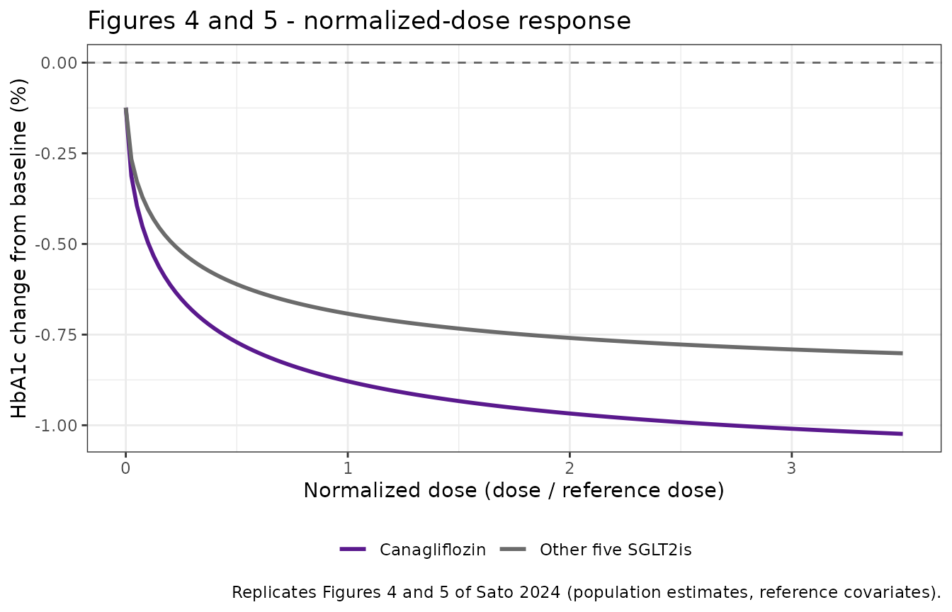
oth <- curves |> filter(Group == "Other five SGLT2is")
can <- curves |> filter(Group == "Canagliflozin")
stopifnot(
  # Curve starts at the placebo value and is monotone downward (deterministic).
  abs(oth$Cc[1] - (-0.124)) < 1e-10,
  all(diff(oth$Cc) <= 1e-12),
  # Canagliflozin is below the others everywhere except at dose 0.
  abs(can$Cc[1] - oth$Cc[1]) < 1e-10,
  all(can$Cc[-1] < oth$Cc[-1])
)
Between-study variability
Variability in this model is between-study, not
between-subject: each draw is a hypothetical new trial arm, not a new
patient. The two etas are correlated (0.785) and act on different scales
– additive on Base, exponential on Emax.
# 200 simulated study arms at the clinical normalized dose of ~1. Residual
# error is zeroed (see Assumptions) but the between-study etas are retained.
mod_isv <- rxode2::zeroRe(mod, "sigma")

isv_arms <- ref_arm(200L)
isv_arms$DOSE_EMPA_MGD <- 11.8
isv <- rxode2::rxSolve(mod_isv, isv_arms, returnType = "data.frame")

ggplot(data.frame(Cc = isv$Cc), aes(Cc)) +
  geom_histogram(bins = 30, fill = "grey70", colour = "white") +
  geom_vline(xintercept = -0.692, colour = "red", linetype = "dashed", linewidth = 1) +
  labs(x = "Study-arm mean HbA1c change (%)", y = "Simulated study arms",
       title = "Between-study variability at normalized dose 1",
       caption = "Red line: the population estimate of -0.692% printed by Sato 2024.") +
  theme_bw()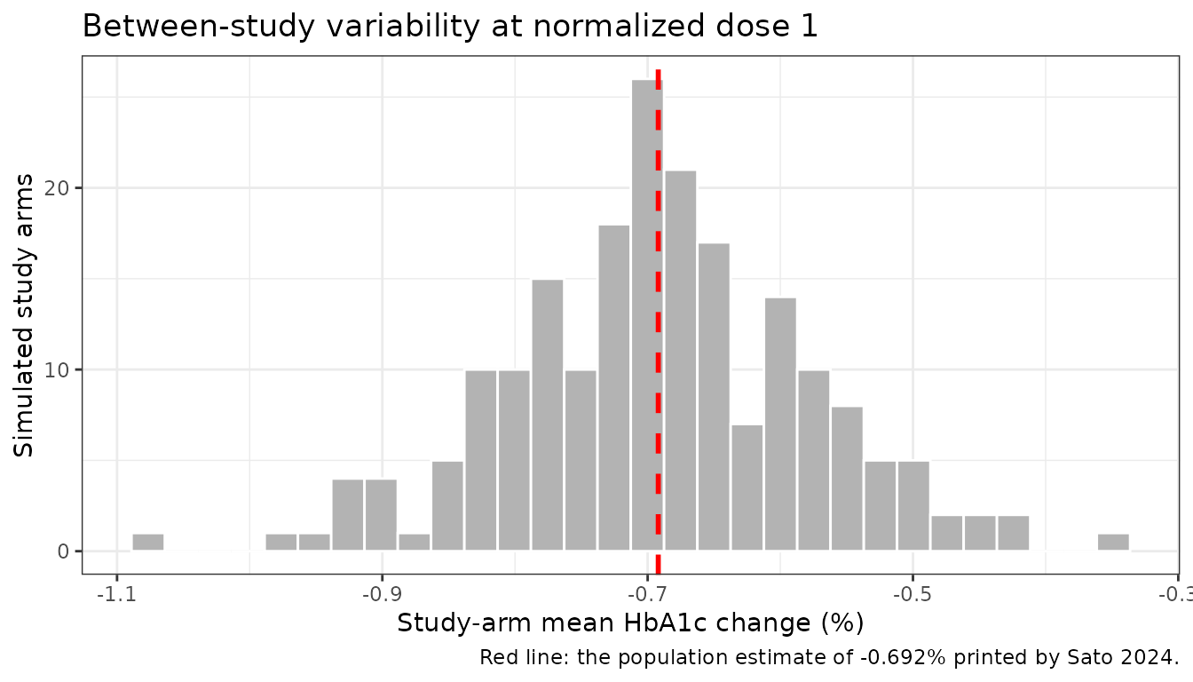
# Cohort-derived quantities: assert only what holds for ANY draw the model can
# produce. omega(Base) = 0.191 additive and omega(Emax) = 0.214 exponential
# give a between-study SD around 0.2-0.3 points at this dose; the bounds below
# sit well outside that spread but still break if an omega were mis-scaled by
# the classic variance-vs-SD factor (which would roughly double the spread) or
# if the location were wrong.
stopifnot(
  nrow(isv) == 200L,
  abs(median(isv$Cc) - (-0.692)) < 0.25,
  sd(isv$Cc) > 0.05, sd(isv$Cc) < 0.75
)
Goodness of fit against the 295 published study arms
As an end-to-end check performed during extraction, the packaged model was run against every study arm in Sato 2024 Supplementary Table S2, using each arm’s own reported covariates, and compared with that arm’s observed mean HbA1c change. This reproduces the paper’s Figure 6a (observations vs population predictions). The supplementary dataset is not redistributed here – the article is CC BY-NC-ND – so the results are reported rather than recomputed.
| Arm set | n | Pearson r | Bias (% HbA1c) | RMSE (% HbA1c) |
|---|---|---|---|---|
| Placebo arms (Base layer only, no imputation) | 70 | 0.35 | +0.025 | 0.217 |
| Active arms with complete covariates (no imputation) | 65 | 0.858 | +0.008 | 0.139 |
| All arms (median imputation for missing covariates) | 295 | 0.884 | +0.001 | 0.173 |
Per-drug bias over all 295 arms was small and unsystematic – canagliflozin +0.001, dapagliflozin -0.041, empagliflozin +0.011, ipragliflozin -0.043, luseogliflozin +0.057, tofogliflozin +0.017 points. That matters beyond a generic fit statistic: a materially wrong reference dose for any one drug would shift that drug’s normalized doses systematically and show up as a drug-specific bias. It does not, which is independent evidence that the six digitized reference doses are right.
The low correlation on the placebo set is expected rather than
alarming: those 70 arms span a narrow range of predictions (only two
distinct values, -0.124 and +0.032, since Base has just one
binary covariate), so the correlation is dominated by residual scatter
while the bias and RMSE remain small.
Assumptions and deviations
-
The six UGE reference doses are digitized from Figure 1, not
printed. This is the only non-paper-derived input in the model,
and it is flagged inline on each
dref_*parameter. Sato 2024 defines them via Eq. 1-4 but publishes them only as the red dashed lines in Figure 1; thedata_uge.csvinput to the authors’ script (Supplementary File MOESM1) is not distributed. Recovery used a 600-dpi render, locating the red dashed line against the x-axis tick calibration (tick-fit residual at most 0.3 mg). Two independent cross-checks agree: extracting the fitted curve and solving it at 51.4 g/day reproduces every reference dose within 1.7%, and locating the clinical-dose markers by their exact palette colours recovers the known clinical doses to within 0.1-1%. Residual digitization error of order 1-2% propagates proportionally to the normalized dose; for context, the bootstrap 95% CI onED50spans 0.191-1.09, a better-than-fourfold range, so the digitization is far from the dominant uncertainty. The 295-arm goodness-of-fit above provides an independent per-drug check. -
The residual is unit-weight and must be scaled per
arm. Sato 2024 fixes the residual sigma at 1 and scales it by
each arm’s standard error,
SD_arm / sqrt(n_arm)(Eq. 6). That weight is a property of each published arm, not of the model, so it cannot live inini(); the model encodesaddSd <- fixed(1)exactly as the paper fixes it, matching the convention used by the other size-weighted MBMAs in this package. A bare stochasticrxSolve()therefore applies a 1-point additive residual, roughly 10-40x too large for a real arm. Scale by the arm’s own standard error, or zero the residual withrxode2::zeroRe(mod, "sigma")as this vignette does. - Between-study, not between-subject. The etas are study-level. The model simulates study-arm mean outcomes and must not be used for individual-patient simulation.
-
Treatment history is encoded with the canonical
TRT_T2DM_*family. Sato 2024 carries two separate binary flags (drug-naive, and any concomitant antihyperglycemic medication) rather than a single four-level stratum. They never co-occur across the 295 arms (51 naive / 53 non-naive / 191 add-on), soTRT_T2DM_NAIVEandTRT_T2DM_ADDONreproduce the encoding exactly andTRT_T2DM_MIXEDis unused. Note that the two act on different parameters here – naive onEmax, add-on onBase. -
The Supplementary Table S2 column headed “Pre-treatment”
actually codes drug-naive. Three independent lines of evidence:
the authors’ own script reads it as
NAIVE = \Drug naive``; the arms coded 1 are the drug-naive trials while insulin add-on trials are coded 0; and the Results text attributes the greater effect to “no prior treatment”. Table 2B’s “Pre-treatment … No: 1.230” is consistent with all three. - Sato 2024 Table 2B misprints the unit of baseline HbA1c as “mg dL-1”. It is NGSP percent – confirmed by the tabulated 7.2-9.1 covariate range and by the Supplementary Table S2 column header “Baseline HbA1c (%)”.
-
The diabetes-duration coefficient is printed with
inconsistent signs. Supplementary Table S3 lists it as +0.025
in its “Original data” half and -0.0247 (95% CI -0.041 to -0.0054) in
its bootstrap half. The function is unambiguous: Table 2B
prints
f(COV) = 1 - 0.025 (COV - 6.6), whose printed range 1.16-0.71 over 0.25-18.2 years reproduces exactly. The model encodes the bootstrap’s signed parameterization1 + theta (COV - 6.6)withtheta = -0.025, numerically identical to the printed form. -
The diabetes-duration effect is linear and must not be
extrapolated.
1 - 0.025 (COV - 6.6)crosses zero at 46.6 years and reverses the sign of the drug effect beyond that. It is only meaningful inside roughly the observed 0.25-18.2 year range. -
Missing covariates in the source dataset are
unexplained. Supplementary Table S2 leaves eGFR blank for 132
of 295 arms, diabetes duration for 93 and body weight for 9, and the
authors’ script writes the NONMEM dataset with
na = "-99". How the stepwise covariate search handled those records is not stated, and theconfig.scmfile the Methods points to is not among the distributed supplementary files. This affects reproduction of the fit, not use of the published model, whose parameters are fully reported. -
ED50is the paper’s own acknowledged weak point. The bootstrap gave a mean of 0.495 against a point estimate of 0.251 and an SE of 3.22. The authors argue the outlying draws paired with small Hill coefficients so the resulting curves stayed similar, and conclude a simpler model than the sigmoid Emax would have sufficed. The point estimate is used here. - No time course. Study duration was screened as a covariate and not retained, so the model predicts the end-of-treatment change for any trial of at least 12 weeks (the pool spans 12-104 weeks) with no time argument.
-
Screened-but-unused covariates (age, sex, BMI,
fasting plasma glucose, systolic and diastolic blood pressure, study
duration, conducted-in-Japan) are recorded in the model’s
covariatesDataExcludedmetadata rather thancovariateData, since the paper reports no point estimate for any of them.