Ceftazidime/avibactam + fosfomycin against multidrug-resistant E. coli (Kroemer 2024)
Source:vignettes/articles/Kroemer_2024_ceftazidime_avibactam_fosfomycin.Rmd
Kroemer_2024_ceftazidime_avibactam_fosfomycin.RmdModel and source
- Article: https://doi.org/10.1128/spectrum.03318-23
- Supplemental material (Text S1-S5, Fig. S1-S2, Tables S1-S4): same
DOI, file
spectrum.03318-23-s0001.docx. The structural equations (Text S3 Eqs 1-13) and every parameter estimate (Tables S3 and S4) live in the supplement; the main text carries no parameter table.
tkc  <- rxode2::rxode(readModelDb("Kroemer_2024_ceftazidime_avibactam_fosfomycin_tkc"))
#> ℹ parameter labels from comments will be replaced by 'label()'
hfim <- rxode2::rxode(readModelDb("Kroemer_2024_ceftazidime_avibactam_fosfomycin_hfim"))
#> ℹ parameter labels from comments will be replaced by 'label()'
cat(tkc$reference, sep = "\n")
#> Kroemer N, Amann LF, Farooq A, Pfaffendorf C, Martens M, Decousser JW, Gregoire N, Nordmann P, Wicha SG. Pharmacokinetic/pharmacodynamic analysis of ceftazidime/avibactam and fosfomycin combinations in an in vitro hollow fiber infection model against multidrug-resistant Escherichia coli. Microbiol Spectr. 2024 Jan;12(1):e03318-23. doi:10.1128/spectrum.03318-23. Structural equations: supplemental material Text S3 Eqs 1-8. Parameter estimates: supplemental material Table S3 (with 95% confidence intervals from sampling importance resampling).
Kroemer 2024 develops two semi-mechanistic PK/PD models of the same clinical multidrug-resistant Escherichia coli isolate, fitted to two different experimental systems, and reports each with its own parameter table and its own visual predictive check:
-
Kroemer_2024_ceftazidime_avibactam_fosfomycin_tkc– the static time-kill model (Text S3 Eqs 1-8, Table S3, VPC in Fig. 1). Two bacterial subpopulations, static drug concentrations supplied as covariates. -
Kroemer_2024_ceftazidime_avibactam_fosfomycin_hfim– the dynamic hollow fiber model (Text S3 Eqs 3-13, Table S4, VPC in Fig. 2). The static model extended with two phenotypically less susceptible subpopulations, and with dosable, decaying antibiotic concentration states.
The hollow fiber model inherits all drug-effect parameters from the static model (“FIX to TKC parameter” throughout Table S4), but it is not a mere re-fit: it adds four parameters’ worth of new structure, re-estimates the carrying capacity and the resistant inoculum, and changes the variability model. Both are published final models, so both are packaged, following the library’s replicate-the-author’s-structure policy. Per that policy this is still one vignette, because it walks one paper.
This is not a population PK model. In the static model the drug concentrations are experimental constants; in the hollow fiber model they are nominal profiles the user doses. There is no absorption-distribution-elimination profile of a drug to integrate, so PKNCA is not the right validation target and the mechanistic checks below replace it.
Population (biological context)
A single clinical E. coli isolate, recovered from a rectal swab during routine multidrug-resistance screening at Henri-Mondor Hospital (Paris). Whole-genome sequencing (shovill v1.0.4 assembly, ResFinder resistome) identified CTX-M-15 and TEM-4 extended-spectrum beta-lactamases and the OXA-244 (OXA-48-like) carbapenemase. It is E. coli YAL_AMA of Kroemer et al. 2023.
MICs by broth microdilution (modal value of triplicates), with fosfomycin also by agar dilution: ceftazidime 16 mg/L, ceftazidime/avibactam 0.125 mg/L, fosfomycin 16/0.5 mg/L. By EUCAST the isolate is susceptible to ceftazidime/avibactam and to fosfomycin, and resistant to ceftazidime alone.
Both experimental systems used cation-adjusted Mueller-Hinton broth 2 at 37 degrees C in ambient air, with 25 mg/L glucose-6-phosphate wherever fosfomycin was present (EUCAST recommendation), an inoculum of 10^6 CFU/mL, and 2 h of preincubation before the first drug exposure:
- Static time-kill: 30 h, 10 mL, counts at 0, 2, 4, 8, 24 and 30 h after drug addition, performed in duplicate. Quantification limit about 101-102 CFU/mL; non-quantifiable counts were set to 1 CFU/mL and kept in the fit.
- Dynamic hollow fiber: 72 h, FiberCell C2011 polysulfone cartridge with a 200 mL central compartment and a 40 mL inoculated extra-capillary space, medium exchanged at 0.834-1.28 mL/min to control the drug elimination. Total counts and counts on 3x MIC drug-supplemented agar were both quantified. Each hollow fiber experiment was run once.
The same information is available programmatically via
readModelDb("Kroemer_2024_ceftazidime_avibactam_fosfomycin_tkc")$population
and its _hfim sibling.
Source trace
Per-parameter origins are recorded as in-file comments next to each
ini() entry in both model files. The tables below collect
them in one place.
Static time-kill model (Table S3)
| Parameter | Value | Source location |
|---|---|---|
log10inoc_s |
6.86 | Table S3, inoculum susceptible (S) |
log10inoc_r |
3.14 | Table S3, inoculum resistant (R) |
log10bmax |
8.92 | Table S3, maximum bacterial capacity |
kgs |
1.81 | Table S3, growth rate (S) |
kgr |
0.45 | Table S3, growth rate (R) |
emax_caz_s, ec50_caz_s,
hill_caz_s
|
3.40, 5.31, 2.32 | Table S3, CAZ on (S) |
emax_caz_r, ec50_caz_r,
hill_caz_r
|
0.659, 74.40, 8.45 | Table S3, CAZ on (R) |
emax_avi_s, ec50_avi_s,
hill_avi_s
|
3.3, 22.3, 1.13 | Table S3, AVI on (S) |
slope_avi_r, hill_avi_r
|
0.0787, 0.317 | Table S3, AVI on (R) (power model) |
slope_fof_s, hill_fof_s
|
2.71, 0.333 | Table S3, FOF on (S) (power model) |
emax_fof_r, ec50_fof_r,
hill_fof_r
|
0.635, 4.70, 4.08 | Table S3, FOF on (R) |
lint_avi_caz_s, lec50int_avi_caz_s,
hillint_avi_caz_s
|
-6.70, -16.20, 0.266 | Table S3, AVI affecting CAZ on (S); footnotes 1-2 give the log-scale back-transforms |
lint_avi_caz_r, lec50int_avi_caz_r,
hillint_avi_caz_r
|
-13.50, -5.23, 1 FIXED | Table S3, AVI affecting CAZ on (R); footnote 3 fixes the Hill factor |
lint_caz_fof_r, lec50int_caz_fof_r,
hillint_caz_fof_r
|
-7.85, -12.40, 0.239 | Table S3, CAZ affecting FOF on (R) |
etalog10inoc_r |
0.108787 | Table S3, 33.9 %CV; footnote 4 gives omega^2 = log(CV^2 + 1) |
etakgr |
0.049810 | Table S3, 22.6 %CV; footnote 4 |
addSd |
1.30 | Table S3, additive residual variability sigma |
| Growth / kill ODEs | n/a | Text S3 Eqs 1-2 |
| Sigmoidal Emax and power effect forms | n/a | Text S3 Eqs 3-4 |
| Bliss independence (3-drug, and its collapse to addition) | n/a | Text S3 Eqs 5-7 |
| GPDI interaction term | n/a | Text S3 Eq 8 |
Dynamic hollow fiber model (Table S4)
Every mono-drug and interaction parameter above is carried over
unchanged and marked fixed() in the model file (“FIX to TKC
parameter” in Table S4). The rows below are what Table S4 adds or
re-estimates.
| Parameter | Value | Source location |
|---|---|---|
log10inoc_s |
6.86 FIXED | Table S4, FIX to TKC parameter |
log10inoc_r |
2.89 | Table S4, re-estimated (lower than the static 3.14) |
log10bmax |
9.73 | Table S4, re-estimated |
kgs, kgr
|
1.81, 0.45 FIXED | Table S4, FIX to TKC parameter |
log10inoc_rcza |
-18 FIXED | Table S4, footnote 3 “fixed to final estimate” |
log10inoc_rfof |
-2.15 | Table S4, inoculum FOF less susceptible |
kgr2 |
2.37 | Table S4, growth rate of both less susceptible subpopulations (merged to one parameter, Text S5) |
ec50_cza_rcza, hill_cza_rcza
|
0.576, 1 FIXED | Table S4, CZA suppressing the CZA less susceptible subpopulation |
ec50_fof_rcza, hill_fof_rcza
|
1.38, 20 FIXED | Table S4, FOF suppressing the CZA less susceptible subpopulation |
ec50_fof_rfof, hill_fof_rfof
|
6.84, 20 FIXED | Table S4, FOF suppressing the FOF less susceptible subpopulation |
ec50_cza_rfof, hill_cza_rfof
|
0.049, 2.49 | Table S4, CZA suppressing the FOF less susceptible subpopulation |
etalog10inoc_r |
0.208826 | Table S4, 48.2 %CV; footnote 5 |
etalog10inoc_rcza |
0.204927 | Table S4, 47.7 %CV; footnote 5 |
addSd |
3.28 | Table S4, additive residual variability on the total count |
addSd_CFUrcza, addSd_CFUrfof
|
0.906, 0.906 | Table S4, one shared additive residual sigma on the less susceptible counts (Text S5); split into two identical entries because rxode2 needs one residual parameter per endpoint |
thalf |
1.81 FIXED | Main-text Table 1, modal simulated half-life (range 1.81-3.03 h); Discussion, “a then-joint elimination half-life of approximately 2 h” |
| Four-subpopulation ODEs | n/a | Text S3 Eqs 9-12 |
| Growth-inhibition (Emax = 1) form | n/a | Text S3 Eq 13 |
Units (dimensional analysis)
| Symbol | Meaning | Units |
|---|---|---|
bact_susceptible, bact_resistant,
bact_resistant_cza, bact_resistant_fof
|
bacterial counts | CFU/mL |
conc_caz, conc_avi, conc_fof,
CONC_*_MGL
|
antibiotic concentrations | mg/L |
kgs, kgr, kgr2,
kel, emax_*, e_s,
e_r
|
rate constants | 1/h |
ec50_*, ec50int_*
|
half-effect concentrations | mg/L |
slope_fof_s, slope_avi_r
|
power-model slopes | (L/mg)^H / h |
hill_*, hillint_*, int_*,
i_*, cap, ea, eb,
ec
|
dimensionless | – |
bmax, inoc_*
|
population scale | CFU/mL |
Every growth and kill term is (1/h) x (CFU/mL) = (CFU/mL)/h, matching
d/dt(state); the drug states are (1/h) x (mg/L) = (mg/L)/h.
The two power models are the one place where the units are carried by
the paper’s parameterisation rather than by a clean rate constant:
slope * C^H must have units 1/h, so
slope_fof_s is (L/mg)^0.333/h and slope_avi_r
is (L/mg)^0.317/h. Table S3 labels both as “L/(mg x h)”, which is the
exact unit only when H = 1; the model file reproduces the published
values and the published functional form.
Parameter tables (paper vs. file)
data.frame(
  parameter = names(tkc$theta),
  value     = unname(tkc$theta)
) |>
  knitr::kable(digits = 6,
caption = "Static time-kill model: typical-value parameters as loaded from the model file (Kroemer 2024 Table S3).")| parameter | value |
|---|---|
| log10inoc_s | 6.8600 |
| log10inoc_r | 3.1400 |
| log10bmax | 8.9200 |
| kgs | 1.8100 |
| kgr | 0.4500 |
| emax_caz_s | 3.4000 |
| ec50_caz_s | 5.3100 |
| hill_caz_s | 2.3200 |
| emax_avi_s | 3.3000 |
| ec50_avi_s | 22.3000 |
| hill_avi_s | 1.1300 |
| slope_fof_s | 2.7100 |
| hill_fof_s | 0.3330 |
| emax_caz_r | 0.6590 |
| ec50_caz_r | 74.4000 |
| hill_caz_r | 8.4500 |
| emax_fof_r | 0.6350 |
| ec50_fof_r | 4.7000 |
| hill_fof_r | 4.0800 |
| slope_avi_r | 0.0787 |
| hill_avi_r | 0.3170 |
| lint_avi_caz_s | -6.7000 |
| lec50int_avi_caz_s | -16.2000 |
| hillint_avi_caz_s | 0.2660 |
| lint_avi_caz_r | -13.5000 |
| lec50int_avi_caz_r | -5.2300 |
| hillint_avi_caz_r | 1.0000 |
| lint_caz_fof_r | -7.8500 |
| lec50int_caz_fof_r | -12.4000 |
| hillint_caz_fof_r | 0.2390 |
| addSd | 1.3000 |
data.frame(
  parameter = names(hfim$theta),
  value     = unname(hfim$theta)
) |>
  knitr::kable(digits = 6,
caption = "Dynamic hollow fiber model: typical-value parameters as loaded from the model file (Kroemer 2024 Table S4).")| parameter | value |
|---|---|
| log10inoc_s | 6.8600 |
| log10inoc_r | 2.8900 |
| log10bmax | 9.7300 |
| kgs | 1.8100 |
| kgr | 0.4500 |
| emax_caz_s | 3.4000 |
| ec50_caz_s | 5.3100 |
| hill_caz_s | 2.3200 |
| emax_avi_s | 3.3000 |
| ec50_avi_s | 22.3000 |
| hill_avi_s | 1.1300 |
| slope_fof_s | 2.7100 |
| hill_fof_s | 0.3330 |
| emax_caz_r | 0.6590 |
| ec50_caz_r | 74.4000 |
| hill_caz_r | 8.4500 |
| emax_fof_r | 0.6350 |
| ec50_fof_r | 4.7000 |
| hill_fof_r | 4.0800 |
| slope_avi_r | 0.0787 |
| hill_avi_r | 0.3170 |
| lint_avi_caz_s | -6.7000 |
| lec50int_avi_caz_s | -16.2000 |
| hillint_avi_caz_s | 0.2660 |
| lint_avi_caz_r | -13.5000 |
| lec50int_avi_caz_r | -5.2300 |
| hillint_avi_caz_r | 1.0000 |
| lint_caz_fof_r | -7.8500 |
| lec50int_caz_fof_r | -12.4000 |
| hillint_caz_fof_r | 0.2390 |
| log10inoc_rcza | -18.0000 |
| log10inoc_rfof | -2.1500 |
| kgr2 | 2.3700 |
| ec50_cza_rcza | 0.5760 |
| hill_cza_rcza | 1.0000 |
| ec50_fof_rcza | 1.3800 |
| hill_fof_rcza | 20.0000 |
| ec50_fof_rfof | 6.8400 |
| hill_fof_rfof | 20.0000 |
| ec50_cza_rfof | 0.0490 |
| hill_cza_rfof | 2.4900 |
| thalf | 1.8100 |
| addSd | 3.2800 |
| addSd_CFUrcza | 0.9060 |
| addSd_CFUrfof | 0.9060 |
Solver note
Four of the published exponents are below 1 (hill_fof_s
= 0.333, hill_avi_r = 0.317, hillint_avi_caz_s
= 0.266, hillint_caz_fof_r = 0.239). The analytic Jacobian
of a C^H term carries a C^(H-1) factor that is
singular at C = 0 (i.e. in every drug-free arm), which the
default BDF solver propagates. All simulations below therefore use the
explicit Dormand-Prince solver, method = "dop853", which
needs no Jacobian.
The hollow fiber model additionally seeds
bact_resistant_cza at 10^-18 CFU/mL and lets it grow across
twenty orders of magnitude, so the absolute tolerance must sit far below
that scale; atol = 1e-16 is used throughout. Because the
model declares three residual endpoints, observation rows carry
dvid = 1 and every rxSolve() call passes
useLinCmt = FALSE (rxode2’s automatic ODE-to-linCmt
conversion otherwise corrupts the dvid-to-compartment mapping).
Carrying-capacity (growth control) check
With no drug present, both models must grow from their inoculum to
the published carrying capacity Bmax and stay there: at the
plateau the logistic term 1 - CFU/Bmax is zero. The static
model was fitted with log10(Bmax) = 8.92 and the hollow
fiber model with log10(Bmax) = 9.73, the larger capacity
reflecting the constant supply of fresh medium in the hollow fiber
system.
tkc_ev_obs <- function(caz, avi, fof, times) {
  data.frame(id = 1L, time = times, evid = 0L, amt = NA_real_,
             cmt = "bact_susceptible",
             CONC_CAZ_MGL = caz, CONC_AVI_MGL = avi, CONC_FOF_MGL = fof)
}

gc_tkc  <- SOLVE(tkc0,  tkc_ev_obs(0, 0, 0, seq(0, 30, by = 0.5)))
gc_hfim <- SOLVE(hfim0, data.frame(id = 1L, time = seq(0, 72, by = 0.5),
                                   evid = 0L, amt = NA_real_,
                                   cmt = "bact_susceptible", dvid = 1L))

cat(sprintf("Static time-kill: log10CFU(0) = %.2f, log10CFU(30) = %.2f  (Bmax = 8.92)\n",
            gc_tkc$log_cfu[gc_tkc$time == 0], gc_tkc$log_cfu[gc_tkc$time == 30]))
#> Static time-kill: log10CFU(0) = 6.86, log10CFU(30) = 8.92  (Bmax = 8.92)
cat(sprintf("Hollow fiber:     log10CFU(0) = %.2f, log10CFU(72) = %.2f  (Bmax = 9.73)\n",
            gc_hfim$log_cfu[gc_hfim$time == 0], gc_hfim$log_cfu[gc_hfim$time == 72]))
#> Hollow fiber:     log10CFU(0) = 6.86, log10CFU(72) = 9.73  (Bmax = 9.73)

bind_rows(
  transmute(gc_tkc,  time, log10CFU = log_cfu, model = "Static time-kill (Bmax 8.92)"),
  transmute(gc_hfim, time, log10CFU = log_cfu, model = "Hollow fiber (Bmax 9.73)")
) |>
  ggplot(aes(time, log10CFU, colour = model)) +
  geom_line(linewidth = 1) +
  geom_hline(yintercept = c(8.92, 9.73), linetype = 2, colour = "grey50") +
  labs(x = "Time (h)", y = expression(log[10]~CFU/mL), colour = NULL,
       title = "Drug-free growth control",
       caption = "Dashed lines: the published carrying capacities.") +
  theme(legend.position = "bottom")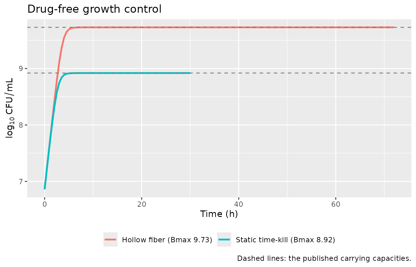
GPDI synergy check
The paper’s central quantitative claim is that the interaction terms reduce the victim drug’s EC50 by more than 99% (Results, “PKPD modeling to quantify synergy”; Text S5). Because both the maximum interaction shift and the interaction potency were estimated on the log scale (Table S3 footnotes 1-2), the claim is worth re-deriving from the tabulated thetas rather than taken on trust.
gpdi_shift <- function(l_int, l_ec50int, h_int, conc) {
  int     <- exp(l_int) - 1        # Table S3 footnote 1
  ec50int <- exp(l_ec50int)        # Table S3 footnote 2
  1 + int * conc^h_int / (ec50int^h_int + conc^h_int)
}

avi_conc <- c(0, 0.4, 1.67, 4, 8.71, 64)
data.frame(
  `Avibactam (mg/L)`  = avi_conc,
  `CAZ EC50 on S`     = 5.31  * gpdi_shift(-6.70,  -16.20, 0.266, avi_conc),
  `CAZ EC50 on R`     = 74.40 * gpdi_shift(-13.50, -5.23,  1,     avi_conc),
  check.names = FALSE
) |>
  knitr::kable(digits = 4,
caption = "Avibactam collapses the ceftazidime EC50 (baselines 5.31 and 74.40 mg/L). At 4 mg/L avibactam -- the concentration used on the ceftazidime agar plates -- the effective EC50 on the susceptible subpopulation falls to about 0.055 mg/L, consistent with the measured ceftazidime/avibactam MIC of 0.125 mg/L against a ceftazidime-alone MIC of 16 mg/L.")| Avibactam (mg/L) | CAZ EC50 on S | CAZ EC50 on R |
|---|---|---|
| 0.00 | 5.3100 | 74.4000 |
| 0.40 | 0.0960 | 0.9827 |
| 1.67 | 0.0680 | 0.2378 |
| 4.00 | 0.0554 | 0.0995 |
| 8.71 | 0.0463 | 0.0458 |
| 64.00 | 0.0300 | 0.0063 |
caz_conc <- c(0, 0.09, 0.87, 1.83, 7.33, 29.06)
data.frame(
  `Ceftazidime (mg/L)` = caz_conc,
  `FOF EC50 on R`      = 4.70 * gpdi_shift(-7.85, -12.40, 0.239, caz_conc),
  `Percent reduction`  = 100 * (1 - gpdi_shift(-7.85, -12.40, 0.239, caz_conc)),
  check.names = FALSE
) |>
  knitr::kable(digits = 4,
caption = "Ceftazidime collapses the fosfomycin EC50 on the resistant subpopulation (baseline 4.70 mg/L). This is the monodirectional GPDI implementation the paper selected (dAIC -271.991 against Bliss independence; Text S5).")| Ceftazidime (mg/L) | FOF EC50 on R | Percent reduction |
|---|---|---|
| 0.00 | 4.7000 | 0.0000 |
| 0.09 | 0.3969 | 91.5558 |
| 0.87 | 0.2399 | 94.8955 |
| 1.83 | 0.2028 | 95.6850 |
| 7.33 | 0.1478 | 96.8544 |
| 29.06 | 0.1078 | 97.7062 |
cat(sprintf("Maximum EC50 reduction, AVI on CAZ (S): %.3f%%\n", 100 * (1 - exp(-6.70))))
#> Maximum EC50 reduction, AVI on CAZ (S): 99.877%
cat(sprintf("Maximum EC50 reduction, AVI on CAZ (R): %.5f%%\n", 100 * (1 - exp(-13.50))))
#> Maximum EC50 reduction, AVI on CAZ (R): 99.99986%
cat(sprintf("Maximum EC50 reduction, CAZ on FOF (R): %.3f%%\n", 100 * (1 - exp(-7.85))))
#> Maximum EC50 reduction, CAZ on FOF (R): 99.961%
All three maximum shifts exceed 99%, matching the paper’s statement that the interactions reduce the EC50 “by >99% for both interacting drug pairs”.
Replicate the static time-kill experiments (Figure 1)
Figure 1 of Kroemer 2024 is a stratified VPC of the static time-kill scenarios. The narrative in Results, “Static time-kill experiments”, states the outcome for each key arm, and those statements are the check applied here: 128 mg/L ceftazidime or 16 mg/L fosfomycin alone were needed for reproducible suppression over 30 h; no avibactam concentration alone killed; 0.125/4 mg/L ceftazidime/avibactam was efficacious; and adding 2 mg/L fosfomycin brought the efficacious ceftazidime concentration down to 0.002 mg/L.
tkc_scenarios <- tribble(
  ~label,                            ~caz,   ~avi, ~fof,
  "Growth control",                   0,      0,    0,
  "CAZ 16 (MIC)",                     16,     0,    0,
  "CAZ 128",                          128,    0,    0,
  "AVI 4",                            0,      4,    0,
  "AVI 64",                           0,      64,   0,
  "FOF 2",                            0,      0,    2,
  "FOF 16 (MIC)",                     0,      0,    16,
  "CZA 0.125/4",                      0.125,  4,    0,
  "CZA 0.002/4",                      0.002,  4,    0,
  "CZA 0.002/4 + FOF 2",              0.002,  4,    2
) |>
  mutate(id = row_number())

tkc_ev <- tkc_scenarios |>
  tidyr::crossing(time = seq(0, 30, by = 0.5)) |>
  transmute(id, time, evid = 0L, amt = NA_real_, cmt = "bact_susceptible",
            CONC_CAZ_MGL = caz, CONC_AVI_MGL = avi, CONC_FOF_MGL = fof)

tkc_sim <- SOLVE(tkc0, tkc_ev) |>
  left_join(select(tkc_scenarios, id, label), by = "id") |>
  mutate(label = factor(label, levels = tkc_scenarios$label))
#> Warning: multi-subject simulation without without 'omega'

ggplot(tkc_sim, aes(time, log_cfu)) +
  geom_line(linewidth = 0.8, colour = "steelblue") +
  geom_hline(yintercept = 0, linetype = 3, colour = "grey60") +
  facet_wrap(~ label, ncol = 3) +
  scale_x_continuous(breaks = seq(0, 30, by = 10)) +
  labs(x = "Time (h)", y = expression(log[10]~CFU/mL),
       title = "Replicates the static time-kill arms of Figure 1 (Kroemer 2024)",
       caption = paste("Typical-value predictions (inter-experimental variability zeroed).",
                       "Dotted line: 1 CFU/mL, the value assigned to non-quantifiable counts."))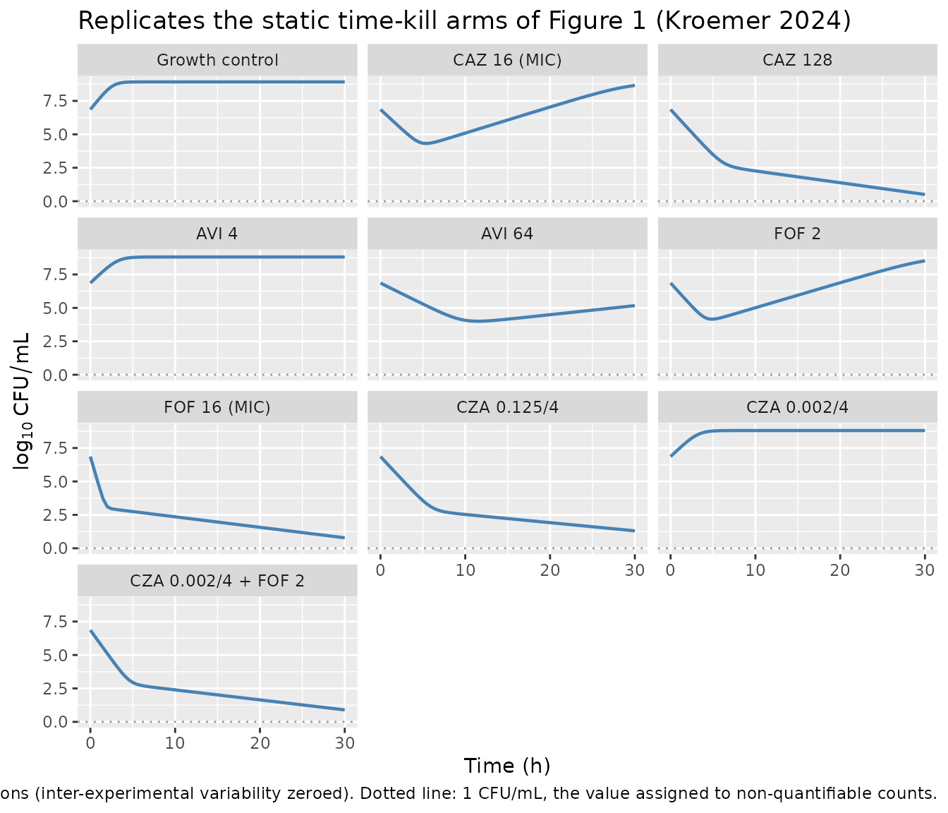
tkc_sim |>
  filter(time == 30) |>
  transmute(Scenario = label, `log10 CFU/mL at 30 h` = log_cfu) |>
  arrange(`log10 CFU/mL at 30 h`) |>
  knitr::kable(digits = 2,
caption = "Bacterial count at the end of the 30-h static time-kill experiment. Suppression (CAZ 128, FOF 16, CZA 0.125/4, CZA 0.002/4 + FOF 2) and regrowth (CAZ 16, FOF 2, avibactam alone at any concentration) reproduce the outcomes reported in Results, 'Static time-kill experiments'.")| Scenario | log10 CFU/mL at 30 h |
|---|---|
| CAZ 128 | 0.50 |
| FOF 16 (MIC) | 0.78 |
| CZA 0.002/4 + FOF 2 | 0.89 |
| CZA 0.125/4 | 1.31 |
| AVI 64 | 5.17 |
| FOF 2 | 8.52 |
| CAZ 16 (MIC) | 8.66 |
| CZA 0.002/4 | 8.81 |
| AVI 4 | 8.81 |
| Growth control | 8.92 |
Replicate the hollow fiber experiments (Figure 2)
Table 1 of the paper gives the simulated steady-state Cmax and Cmin
of every hollow fiber arm. Because the drugs were given as bolus
injections into a one-compartment system, dosing the concentration
increment Cmax - Cmin every 8 h reproduces the published
envelope exactly.
hfim_arms <- tribble(
  ~label,                        ~caz_min, ~caz_max, ~avi_min, ~avi_max, ~fof_min, ~fof_max,
  "Growth control",                  0,       0,        0,       0,        0,       0,
  "CZA 2/0.5 g q8h 50th",            5.70,    41.11,    1.43,    8.71,     0,       0,
  "CZA 2/0.5 g q8h 5th",             1.40,    29.06,    0.32,    6.69,     0,       0,
  "CZA 1/0.25 g q8h 5th",            0.71,    14.66,    0.16,    3.34,     0,       0,
  "CZA 0.5/0.125 g q8h 5th",         0.35,    7.33,     0.08,    1.67,     0,       0,
  "CZA 0.125/0.03 g q8h 5th",        0.09,    1.83,     0.02,    0.40,     0,       0,
  "FOF 6 g q8h 5th",                 0,       0,        0,       0,        13.67,   185.37,
  "FOF 4 g q8h 5th",                 0,       0,        0,       0,        6.74,    124.31,
  "FOF 1 g q8h 5th",                 0,       0,        0,       0,        1.68,    31.08,
  "FOF 0.25 g q8h 5th",              0,       0,        0,       0,        0.37,    7.72,
  "CZA 0.5/0.125 + FOF 1 g q8h",     0.35,    7.33,     0.08,    1.67,     1.50,    31.12,
  "CZA 0.125/0.03 + FOF 0.25 g q8h", 0.09,    1.83,     0.02,    0.40,     0.37,    7.72
) |>
  mutate(id = row_number())

HFIM_DUR <- 72

# One bolus per 8-h interval, sized as the Table 1 concentration increment.
hfim_doses <- hfim_arms |>
  select(id, caz_min, caz_max, avi_min, avi_max, fof_min, fof_max) |>
  pivot_longer(-id, names_to = c("drug", ".value"), names_sep = "_") |>
  filter(max > 0) |>
  mutate(cmt = paste0("conc_", drug), amt = max - min) |>
  tidyr::crossing(time = seq(0, HFIM_DUR - 1, by = 8)) |>
  transmute(id, time, evid = 1L, amt, cmt, dvid = NA_integer_)

hfim_obs <- hfim_arms |>
  select(id) |>
  tidyr::crossing(time = seq(0, HFIM_DUR, by = 0.5)) |>
  transmute(id, time, evid = 0L, amt = NA_real_,
            cmt = "bact_susceptible", dvid = 1L)

hfim_ev <- bind_rows(hfim_obs, hfim_doses) |> arrange(id, time, evid)

hfim_sim <- SOLVE(hfim0, hfim_ev) |>
  left_join(select(hfim_arms, id, label), by = "id") |>
  mutate(label = factor(label, levels = hfim_arms$label))
#> Warning: multi-subject simulation without without 'omega'
hfim_sim |>
  filter(time %in% c(64, 72)) |>
  group_by(label) |>
  summarise(`CAZ Cmin` = min(conc_caz), `CAZ Cmax` = max(conc_caz),
            `AVI Cmin` = min(conc_avi), `AVI Cmax` = max(conc_avi),
            `FOF Cmin` = min(conc_fof), `FOF Cmax` = max(conc_fof),
            .groups = "drop") |>
  knitr::kable(digits = 2,
caption = "Simulated steady-state trough (t = 64 h, just before the ninth dose) and peak (t = 72 h) concentrations, to be compared with Table 1 of the paper.")| label | CAZ Cmin | CAZ Cmax | AVI Cmin | AVI Cmax | FOF Cmin | FOF Cmax |
|---|---|---|---|---|---|---|
| Growth control | 0.00 | 0.00 | 0.00 | 0.00 | 0.00 | 0.00 |
| CZA 2/0.5 g q8h 50th | 1.74 | 37.15 | 0.36 | 7.64 | 0.00 | 0.00 |
| CZA 2/0.5 g q8h 5th | 1.36 | 29.02 | 0.31 | 6.68 | 0.00 | 0.00 |
| CZA 1/0.25 g q8h 5th | 0.68 | 14.63 | 0.16 | 3.34 | 0.00 | 0.00 |
| CZA 0.5/0.125 g q8h 5th | 0.34 | 7.32 | 0.08 | 1.67 | 0.00 | 0.00 |
| CZA 0.125/0.03 g q8h 5th | 0.09 | 1.83 | 0.02 | 0.40 | 0.00 | 0.00 |
| FOF 6 g q8h 5th | 0.00 | 0.00 | 0.00 | 0.00 | 8.41 | 180.11 |
| FOF 4 g q8h 5th | 0.00 | 0.00 | 0.00 | 0.00 | 5.76 | 123.33 |
| FOF 1 g q8h 5th | 0.00 | 0.00 | 0.00 | 0.00 | 1.44 | 30.84 |
| FOF 0.25 g q8h 5th | 0.00 | 0.00 | 0.00 | 0.00 | 0.36 | 7.71 |
| CZA 0.5/0.125 + FOF 1 g q8h | 0.34 | 7.32 | 0.08 | 1.67 | 1.45 | 31.07 |
| CZA 0.125/0.03 + FOF 0.25 g q8h | 0.09 | 1.83 | 0.02 | 0.40 | 0.36 | 7.71 |
The twelve arms driven by the model’s default 1.81-h half-life
reproduce their Table 1 Cmin / Cmax pairs closely
(e.g. CZA 2/0.5 g q8h 5th: 1.36 / 29.02 mg/L here against
1.40 / 29.06 mg/L published). The two arms that Table 1 assigns a
different half-life are visibly off at the trough, exactly as
expected: CZA 2/0.5 g q8h 50th was run at 3.03 h and
FOF 6 g q8h 5th at 2.10 h, so their simulated troughs here
(1.74 and 8.41 mg/L) fall below the published 5.70 and 13.67 mg/L.
Reproducing those two arms exactly requires overriding
thalf; see Assumptions item 5.
hfim_long <- hfim_sim |>
  select(id, label, time, Total = log_cfu, `3x MIC CZA-R` = CFUrcza, `3x MIC FOF-R` = CFUrfof) |>
  pivot_longer(c(Total, `3x MIC CZA-R`, `3x MIC FOF-R`),
               names_to = "population", values_to = "log10CFU") |>
  # The paper plots counts on the observed scale, where non-quantifiable
  # samples were assigned 1 CFU/mL (0 log10). Clamp the total for display only.
  mutate(log10CFU = pmax(log10CFU, 0))

ggplot(hfim_long, aes(time, log10CFU, colour = population)) +
  geom_line(linewidth = 0.7) +
  facet_wrap(~ label, ncol = 3) +
  scale_x_continuous(breaks = seq(0, 72, by = 24)) +
  labs(x = "Time (h)", y = expression(log[10]~CFU/mL), colour = NULL,
       title = "Replicates the hollow fiber arms of Figure 2 (Kroemer 2024)",
       caption = paste("Typical-value predictions. Counts clamped at 0 log10 (1 CFU/mL) for display,",
                       "matching the paper's treatment of non-quantifiable samples.")) +
  theme(legend.position = "bottom")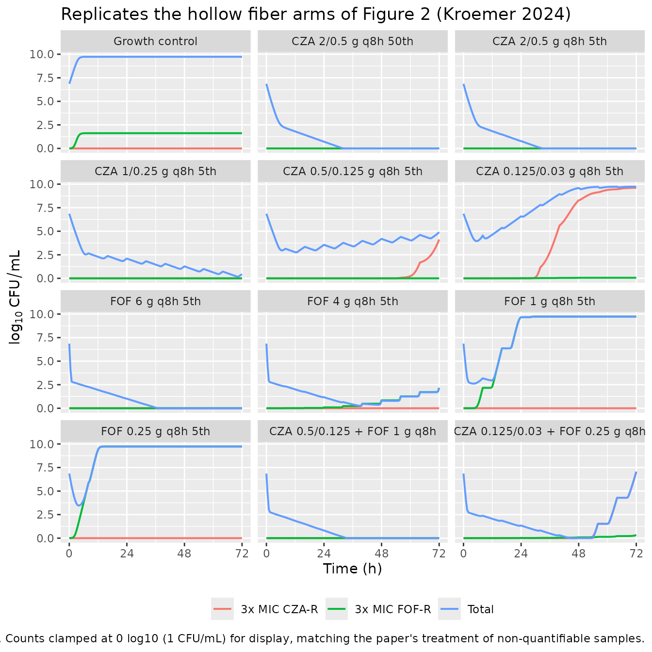
hfim_sim |>
  filter(time == HFIM_DUR) |>
  transmute(Arm = label,
            `Total (log10 CFU/mL)`   = pmax(log_cfu, 0),
            `3x MIC CZA-R`           = CFUrcza,
            `3x MIC FOF-R`           = CFUrfof) |>
  knitr::kable(digits = 2,
caption = "Bacterial counts at 72 h. Results, 'Dynamic HFIM', reports that FOF 1 g q8h was the highest fosfomycin monotherapy that failed to suppress regrowth, that CZA 0.5/0.125 g q8h was the highest ceftazidime/avibactam monotherapy that failed, and that the quarter-dose combination (CZA 0.125/0.03 + FOF 0.25 g q8h) still achieved killing -- all three reproduce here.")| Arm | Total (log10 CFU/mL) | 3x MIC CZA-R | 3x MIC FOF-R |
|---|---|---|---|
| Growth control | 9.73 | 0.00 | 1.62 |
| CZA 2/0.5 g q8h 50th | 0.00 | 0.00 | 0.00 |
| CZA 2/0.5 g q8h 5th | 0.00 | 0.00 | 0.00 |
| CZA 1/0.25 g q8h 5th | 0.44 | 0.00 | 0.00 |
| CZA 0.5/0.125 g q8h 5th | 4.90 | 4.12 | 0.00 |
| CZA 0.125/0.03 g q8h 5th | 9.73 | 9.61 | 0.06 |
| FOF 6 g q8h 5th | 0.00 | 0.00 | 0.00 |
| FOF 4 g q8h 5th | 2.17 | 0.00 | 2.17 |
| FOF 1 g q8h 5th | 9.73 | 0.00 | 9.73 |
| FOF 0.25 g q8h 5th | 9.73 | 0.00 | 9.73 |
| CZA 0.5/0.125 + FOF 1 g q8h | 0.00 | 0.00 | 0.00 |
| CZA 0.125/0.03 + FOF 0.25 g q8h | 7.06 | 7.06 | 0.33 |
The emergence pattern also reproduces the paper’s observation that “below a certain exposure, a rapid emergence of 3x MIC FOF-resistant bacteria was observed within the first 12 h of experiment. On opposite, phenotypic resistance against 3x MIC CZA emerged later between 24 and 48 h”: the fosfomycin less susceptible subpopulation starts from 10^-2.15 CFU/mL and needs only a few hours to become detectable, whereas the ceftazidime/avibactam one starts from 10^-18 CFU/mL and needs roughly 20 h of uninhibited growth at 2.37/h to cross 1 CFU/mL.
emergence <- hfim_sim |>
  group_by(label) |>
  summarise(
    `First time 3x MIC FOF-R > 1 log10 (h)` =
      ifelse(any(CFUrfof > 1), min(time[CFUrfof > 1]), NA_real_),
    `First time 3x MIC CZA-R > 1 log10 (h)` =
      ifelse(any(CFUrcza > 1), min(time[CFUrcza > 1]), NA_real_),
    .groups = "drop"
  )
knitr::kable(emergence, digits = 1,
caption = "Time at which each less susceptible subpopulation first exceeds 10 CFU/mL. NA means the subpopulation never emerged within 72 h.")| label | First time 3x MIC FOF-R > 1 log10 (h) | First time 3x MIC CZA-R > 1 log10 (h) |
|---|---|---|
| Growth control | 3.5 | NA |
| CZA 2/0.5 g q8h 50th | NA | NA |
| CZA 2/0.5 g q8h 5th | NA | NA |
| CZA 1/0.25 g q8h 5th | NA | NA |
| CZA 0.5/0.125 g q8h 5th | NA | 63.0 |
| CZA 0.125/0.03 g q8h 5th | NA | 32.0 |
| FOF 6 g q8h 5th | NA | NA |
| FOF 4 g q8h 5th | 56.0 | NA |
| FOF 1 g q8h 5th | 7.0 | NA |
| FOF 0.25 g q8h 5th | 3.5 | NA |
| CZA 0.5/0.125 + FOF 1 g q8h | NA | NA |
| CZA 0.125/0.03 + FOF 0.25 g q8h | NA | 55.5 |
Inter-experimental variability
Both models carry the paper’s inter-experimental variability as exponential interindividual variability. The hollow fiber model places it on the resistant inoculum (48.2 %CV) and on the ceftazidime/avibactam less susceptible inoculum (47.7 %CV) – the latter is precisely the mechanism the paper introduced to explain why “the lower resistance development against CZA was additionally subjected to a higher variability”, producing “relatively wide prediction intervals in the VPC plots”.
N_SUB <- 100   # participants per arm; well under the 200/arm cap

vpc_arms <- hfim_arms |> filter(label %in% c("CZA 0.5/0.125 g q8h 5th",
                                             "CZA 1/0.25 g q8h 5th"))

vpc_ev <- bind_rows(lapply(seq_len(nrow(vpc_arms)), function(k) {
  arm <- vpc_arms[k, ]
  base_id <- (k - 1L) * N_SUB
  doses <- tidyr::crossing(
    tibble(cmt = c("conc_caz", "conc_avi"),
           amt = c(arm$caz_max - arm$caz_min, arm$avi_max - arm$avi_min)),
    time = seq(0, HFIM_DUR - 1, by = 8),
    sub  = seq_len(N_SUB)
  ) |>
    transmute(id = base_id + sub, time, evid = 1L, amt, cmt, dvid = NA_integer_)
  obs <- tidyr::crossing(sub = seq_len(N_SUB), time = seq(0, HFIM_DUR, by = 2)) |>
    transmute(id = base_id + sub, time, evid = 0L, amt = NA_real_,
              cmt = "bact_susceptible", dvid = 1L)
  bind_rows(obs, doses) |> mutate(arm = arm$label)
}))

vpc_sim <- rxode2::rxSolve(
  hfim, select(vpc_ev, -arm), returnType = "data.frame",
  omega = hfim$omega, method = "dop853", useLinCmt = FALSE,
  maxsteps = 1e7, atol = 1e-16, rtol = 1e-8, keep = character()
) |>
  left_join(distinct(vpc_ev, id, arm), by = "id")

stopifnot(dplyr::n_distinct(vpc_sim$id) == N_SUB * nrow(vpc_arms))

vpc_sim |>
  group_by(arm, time) |>
  summarise(lo = quantile(pmax(log_cfu, 0), 0.05),
            md = median(pmax(log_cfu, 0)),
            hi = quantile(pmax(log_cfu, 0), 0.95), .groups = "drop") |>
  ggplot(aes(time, md)) +
  geom_ribbon(aes(ymin = lo, ymax = hi), alpha = 0.25, fill = "steelblue") +
  geom_line(linewidth = 0.9, colour = "steelblue") +
  facet_wrap(~ arm) +
  scale_x_continuous(breaks = seq(0, 72, by = 24)) +
  labs(x = "Time (h)", y = expression(log[10]~CFU/mL),
       title = "Simulated 90% prediction interval of the total bacterial count",
       caption = paste0("n = ", N_SUB, " simulated experiments per arm; structural variability only ",
                        "(residual error excluded). Compare with the shaded areas of Figure 2."))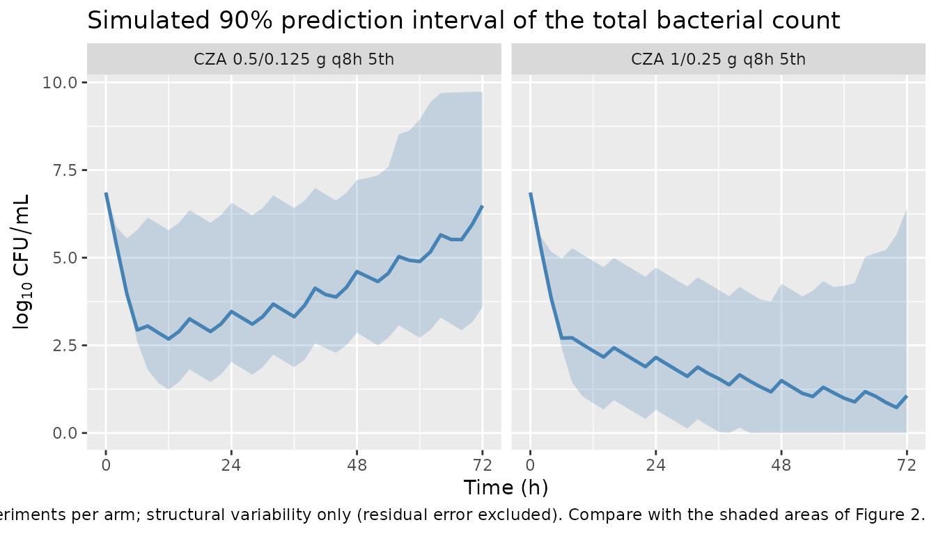
Replicate the dose-response surface (Figure 4)
Figure 4 simulates additional hollow fiber experiments across a grid
of ceftazidime/avibactam and fosfomycin doses and reports the effect
size as the log10 CFU/mL reduction relative to no treatment at 72 h. The
pharmacokinetics in Table 1 are dose-linear, so each grid point is
obtained by scaling the Table 1 reference rows
(CZA 1/0.25 g q8h 5th and
FOF 1 g q8h 5th).
# Table 1 reference rows, per 1 g q8h (5th percentile profiles).
CAZ_PER_G <- c(min = 0.71, max = 14.66)   # CZA 1/0.25 g q8h 5th
AVI_PER_G <- c(min = 0.16, max = 3.34)    # avibactam accompanies at a 4:1 ratio
FOF_PER_G <- c(min = 1.68, max = 31.08)   # FOF 1 g q8h 5th

cza_doses <- c(0, 0.0625, 0.125, 0.25, 0.5, 1, 1.5, 2)
fof_doses <- c(0, 0.125, 0.25, 0.5, 1, 2, 4, 6)

grid <- tidyr::crossing(cza_g = cza_doses, fof_g = fof_doses) |>
  mutate(id = row_number())

grid_doses <- grid |>
  transmute(id,
            conc_caz = cza_g * (CAZ_PER_G[["max"]] - CAZ_PER_G[["min"]]),
            conc_avi = cza_g * (AVI_PER_G[["max"]] - AVI_PER_G[["min"]]),
            conc_fof = fof_g * (FOF_PER_G[["max"]] - FOF_PER_G[["min"]])) |>
  pivot_longer(-id, names_to = "cmt", values_to = "amt") |>
  filter(amt > 0) |>
  tidyr::crossing(time = seq(0, HFIM_DUR - 1, by = 8)) |>
  transmute(id, time, evid = 1L, amt, cmt, dvid = NA_integer_)

grid_obs <- grid |>
  select(id) |>
  tidyr::crossing(time = c(0, 24, 48, 72)) |>
  transmute(id, time, evid = 0L, amt = NA_real_,
            cmt = "bact_susceptible", dvid = 1L)

grid_sim <- SOLVE(hfim0, bind_rows(grid_obs, grid_doses) |> arrange(id, time, evid))
#> Warning: multi-subject simulation without without 'omega'

no_treatment <- grid_sim$log_cfu[grid_sim$id == grid$id[grid$cza_g == 0 & grid$fof_g == 0] &
                              grid_sim$time == HFIM_DUR]

surface <- grid_sim |>
  filter(time == HFIM_DUR) |>
  select(id, log_cfu) |>
  left_join(grid, by = "id") |>
  mutate(effect = no_treatment - pmax(log_cfu, 0))

ggplot(surface, aes(factor(cza_g), factor(fof_g), fill = effect)) +
  geom_tile(colour = "white") +
  geom_text(aes(label = sprintf("%.1f", effect)), size = 2.6) +
  scale_fill_viridis_c(name = "log10 CFU/mL\nreduction") +
  labs(x = "Ceftazidime/avibactam (g ceftazidime q8h)",
       y = "Fosfomycin (g q8h)",
       title = "Replicates the dose-response surface of Figure 4 (Kroemer 2024)",
       caption = "Effect size = log10 CFU/mL reduction versus no treatment at 72 h.")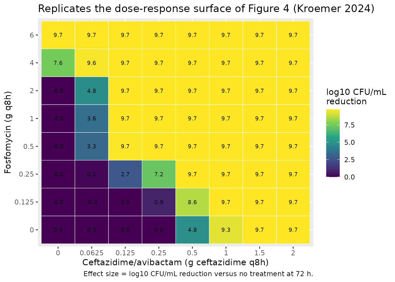
The paper’s headline simulation result is that “a combination of 0.5-g q8h FOF and 0.25-/0.06-g q8h CZA would lead to a suppression of the bacterial count, while a 12 times higher dose of FOF (6 g q8h) or a six times higher dose of CZA (1.5/0.375 g q8h) would lead to the same effects in monotherapy”. The three grid points named in that sentence are compared directly below.
pick <- function(cza, fof) {
  round(surface$effect[surface$cza_g == cza & surface$fof_g == fof], 2)
}
tibble::tibble(
  Regimen = c("Combination: CZA 0.25 g + FOF 0.5 g q8h",
              "Fosfomycin monotherapy: FOF 6 g q8h (12x the combination dose)",
              "CZA monotherapy: CZA 1.5 g q8h (6x the combination dose)"),
  `log10 CFU/mL reduction at 72 h` = c(pick(0.25, 0.5), pick(0, 6), pick(1.5, 0))
) |>
  knitr::kable(digits = 2,
caption = "The paper's dose-reduction claim: a combination of 0.5 g q8h fosfomycin with 0.25/0.06 g q8h ceftazidime/avibactam matches the effect of either monotherapy at 12x (fosfomycin) or 6x (ceftazidime/avibactam) the dose.")| Regimen | log10 CFU/mL reduction at 72 h |
|---|---|
| Combination: CZA 0.25 g + FOF 0.5 g q8h | 9.73 |
| Fosfomycin monotherapy: FOF 6 g q8h (12x the combination dose) | 9.73 |
| CZA monotherapy: CZA 1.5 g q8h (6x the combination dose) | 9.73 |
The three regimens give an identical effect size, but that on its own would also be true of any three regimens strong enough to saturate the endpoint. The sharper test is whether 1.5 g and 6 g really are the smallest monotherapy doses on the simulated grid that reach full suppression – which is what makes the multipliers 6x and 12x rather than merely “at least”.
surface |>
  filter(cza_g == 0 | fof_g == 0) |>
  transmute(
    Monotherapy = ifelse(fof_g == 0 & cza_g == 0, "No treatment",
                  ifelse(fof_g == 0, "Ceftazidime/avibactam", "Fosfomycin")),
    `Dose (g q8h)` = ifelse(fof_g == 0, cza_g, fof_g),
    `log10 CFU/mL reduction at 72 h` = round(effect, 2)
  ) |>
  filter(Monotherapy != "No treatment") |>
  arrange(Monotherapy, `Dose (g q8h)`) |>
knitr::kable(caption = "Monotherapy dose-response at 72 h. Full suppression (a 9.73 log10 reduction, i.e. the whole no-treatment plateau) is first reached at 1.5 g q8h ceftazidime and at 6 g q8h fosfomycin; the next dose down in each series (1 g and 4 g) leaves 0.4 and 2.2 log10 CFU/mL standing. Against the combination's 0.25 g and 0.5 g, those thresholds are the paper's 6-fold and 12-fold dose reductions exactly.")| Monotherapy | Dose (g q8h) | log10 CFU/mL reduction at 72 h |
|---|---|---|
| Ceftazidime/avibactam | 0.0625 | 0.00 |
| Ceftazidime/avibactam | 0.1250 | 0.00 |
| Ceftazidime/avibactam | 0.2500 | 0.00 |
| Ceftazidime/avibactam | 0.5000 | 4.82 |
| Ceftazidime/avibactam | 1.0000 | 9.29 |
| Ceftazidime/avibactam | 1.5000 | 9.73 |
| Ceftazidime/avibactam | 2.0000 | 9.73 |
| Fosfomycin | 0.1250 | 0.00 |
| Fosfomycin | 0.2500 | 0.00 |
| Fosfomycin | 0.5000 | 0.00 |
| Fosfomycin | 1.0000 | 0.00 |
| Fosfomycin | 2.0000 | 0.00 |
| Fosfomycin | 4.0000 | 7.57 |
| Fosfomycin | 6.0000 | 9.73 |
Assumptions and deviations
Eq 2 / Eq 10 kill term reads
- R * E_R, not- S * E_Ras printed. Text S3 prints the resistant compartment’s kill term with the susceptible count as its multiplier, in both the static (Eq 2) and the hollow fiber (Eq 10) equation. Taken literally, at the estimated inocula (10^6.86 vs 10^3.14 CFU/mL) that term is roughly 5,000x larger than the resistant state itself and drives it negative within minutes, and it would also leave the resistant subpopulation entirely uncontrollable once the susceptible one is eradicated – which is the opposite of the paper’s whole argument. Figure 3 of the main text draws the drug effects acting on the resistant bacteria (“dashed arrow, drug effects on the resistant bacteria”), and the semi-mechanistic form the paper builds on (Nielsen 2011, supplement ref 6) is- R * E_R. TheSis read as a typesetting error and implemented asR. The replications above – which reproduce every outcome the Results section states in words – support that reading.The exponential IIV is applied to the log10-scale parameter. Text S5 says inter-experimental variability was “implemented on both parameters as exponential coefficient of variation”, but does not say whether the eta multiplies the tabulated log10 inoculum or the underlying linear CFU count. The log10-scale reading is used (
inoc = 10^(log10inoc * exp(eta))). On the linear-count reading, a 47.7 %CV on the ceftazidime/avibactam less susceptible inoculum would move 10^-18 CFU/mL by well under half a log10 and shift the emergence of resistance by under 15 minutes – far too little to produce the wide prediction intervals that the paper introduced this eta to capture, or the observed 24-48 h spread in the emergence of ceftazidime/avibactam resistance. On the log10 reading the same %CV shifts the emergence by several hours, which matches. Users who need the alternative reading can change the twoinoc_*lines inmodel().The tabulated residual
sigmais taken as a standard deviation. Tables S3 and S4 report “additive residual variability sigma” (1.30 for the static model; 3.28 and 0.906 for the hollow fiber model) in log(CFU/mL), without stating whether the number is the NONMEM$SIGMAvariance or its square root. The values are encoded literally asaddSdstandard deviations, which is what the symbol conventionally denotes. If the tabulated numbers are variances, the corresponding SDs would be 1.14, 1.81 and 0.95. This affects only the residual-error magnitude, not any typical-value prediction, and the VPC above deliberately shows structural variability only.The shared less-susceptible residual sigma is split into two parameters. Text S5 states that the residual errors of the two less susceptible subpopulations “were estimated to be similar. Therefore, they were merged to one respective parameter”. rxode2 requires one residual parameter per endpoint, so
addSd_CFUrczaandaddSd_CFUrfofboth carry the single published estimate of 0.906. A user re-estimating this model should constrain them to be equal to recover the published parameterisation.A joint 1.81-h half-life is used for all three drugs. Table 1 reports a per-experiment simulated half-life ranging from 1.81 to 3.03 h, shared across the three drugs within each experiment; 1.81 h is the value for 11 of the 14 experiments and is used as the model default (
thalf, FIXED). The Discussion describes the design intent as “a simplified control of the elimination of all three drugs with a then-joint elimination half-life of approximately 2 h”. Users reproducing a specific Table 1 arm should overridethalfwith that arm’s value; the two arms at 3.03 h and 2.10 h areCZA 2/0.5 g q8h 50thandFOF 6 g q8h 5th.The hollow fiber pharmacokinetics are dosed as concentration increments. The drugs were given as bolus injections into the 200 mL central compartment and the paper reports only the resulting Cmax and Cmin, not doses in mg. The model carries
conc_caz,conc_aviandconc_fofas concentration states (mg/L), so a dose amount is a concentration increment. DosingCmax - Cminevery 8 h reproduces the Table 1 envelope at steady state, as the concentration table above confirms; the first peak is slightly below the steady-state Cmax, matching the real experiment, which began dosing after 2 h of preincubation.The less susceptible outputs carry a 0 log10 baseline; the total does not. Text S5 states that “to account for the lower limit of quantification of the less susceptible subpopulations a baseline was set to 0 log10(CFU/mL)”.
CFUrczaandCFUrfoftherefore computelog10(state + 1), which sits at 0 until the subpopulation exceeds 1 CFU/mL. No equivalent statement is made for the total count, solog_cfuis the untransformedlog10of the summed state and can fall below 0 under strong killing; the figures above clamp it at 0 for display only, matching the paper’s convention of assigning 1 CFU/mL to non-quantifiable samples.Bliss normalisation on the resistant subpopulation excludes avibactam. Eq 5 normalises the three-drug Bliss expression by the largest mono-drug Emax. Avibactam’s effect on the resistant subpopulation is a power model and so has no Emax; Text S5 states that “just the maximum effects of ceftazidime and fosfomycin were considered for the normalization for the calculation of Bliss Independence on the (R) population”. Avibactam still enters the Bliss expression itself (Eq 6) as the third drug.
Protein binding is not in the model. The Methods assume unbound fractions of 92% (avibactam), 85% (ceftazidime) and effectively 100% (fosfomycin), but the hollow fiber system contains no protein, so the concentrations the model works with are the total concentrations mimicked in broth. The unbound fractions were used upstream when selecting the clinical profiles to mimic, not inside the PK/PD model.
No pharmacokinetic drug interaction between avibactam and ceftazidime. Three modes of avibactam action are conceivable (own kill, potentiation of ceftazidime, suppression of beta-lactamase-mediated ceftazidime degradation). The bioanalysis found no ceftazidime degradation at the avibactam concentrations studied, so the paper assumed permanent beta-lactamase inhibition and modelled only the first two mechanisms. The model files follow that choice.
Single strain, single hollow fiber replicate. The whole analysis rests on one clinical isolate; the static time-kill experiments were duplicated but each hollow fiber arm was run once. The paper is explicit that confirmation across strains “would be desirable”. The variability terms are inter-experimental, not between-patient, and the models should not be used to simulate clinical between-subject variability.