Valganciclovir (Vezina 2010)
Source:vignettes/articles/Vezina_2010_valganciclovir.Rmd
Vezina_2010_valganciclovir.RmdModel and source
- Citation: Vezina HE, Brundage RC, Nevins TE, Balfour HH Jr. The pharmacokinetics of valganciclovir prophylaxis in pediatric solid organ transplant patients at risk for Epstein-Barr virus disease. Clin Pharmacol Adv Appl. 2010;2:1-7. doi:10.2147/CPAA.S8341
- Description: One-compartment population PK model for ganciclovir following oral valganciclovir prophylaxis in pediatric solid organ transplant recipients at risk for Epstein-Barr virus disease (Vezina 2010). First-order absorption with no covariates retained in the final model; doses are mg of valganciclovir uncorrected for molecular weight, and the apparent CL/F and V/F absorb both oral bioavailability and the molar conversion from valganciclovir to ganciclovir.
- Article: https://doi.org/10.2147/CPAA.S8341
Population
The model was developed from 43 ganciclovir plasma concentrations collected from 8 pediatric solid organ transplant recipients enrolled at the University of Minnesota Medical Center / General Clinical Research Center (Vezina 2010 Methods ‘Subjects’ and ‘Study design’, Table 1). Subjects were 1.3 - 6.2 years of age (median 2.1), with body weight 9.4 - 19.8 kg (median 14.1), height 73 - 107 cm (median 89.5), and Schwartz creatinine clearance 61.9 - 127 mL/min/1.73 m^2 (median 106). 25% of subjects (2 of 8) were female. Five received kidney transplants and three received liver transplants. All eight were taking a 90 mg/mL valganciclovir oral suspension compounded by the University of Minnesota Medical Center’s Fairview Specialty Pharmacy, dosed by weight at the median (range) of 11.1 (10.1 - 12.1) mg/kg every 12 hours or 7.4 (5.3 - 11.3) mg/kg every 24 hours, with adjustments for renal function. The study sampled either an intensive 12-hour visit (0, 1, 2, 4, 6, 8, 12 hours post-dose; subjects fasted overnight then received the dose immediately after a standardized 641 kcal breakfast) or two sparse visits during routine transplant clinic appointments; two of the eight subjects participated in both intensive and sparse arms.
The same information is available programmatically via
readModelDb("Vezina_2010_valganciclovir")$population.
Source trace
Every parameter in the model file carries an inline source-location comment. The table below collects the entries in one place.
| Equation / parameter | Value | Source location |
|---|---|---|
lcl (CL/F) |
7.33 L/h | Table 2, Estimate column, CL/F row |
lvc (V/F) |
35.1 L | Table 2, Estimate column, V/F row |
lka (Ka) |
0.85 1/h | Table 2, Estimate column, Ka row |
| IIV CL/F (omega^2 = log(0.363^2 + 1) = 0.1238) | 36.3% CV | Table 2, Estimate column, Variability in CL/F row |
| IIV V/F (omega^2 = log(0.414^2 + 1) = 0.1582) | 41.4% CV | Table 2, Estimate column, Variability in V/F row |
| IIV Ka (omega^2 = log(0.743^2 + 1) = 0.4397) | 74.3% CV | Table 2, Estimate column, Variability in Ka row |
| Proportional residual error | 33.5% CV | Table 2, Estimate column, RUV row |
| Bioavailability F | implicit in CL/F and V/F (apparent) | Methods ‘Pharmacokinetic analysis’ (parameterized as CL/F and V/F throughout) |
| 1-cmt structure with first-order absorption | – | Methods ‘Pharmacokinetic analysis’ (NONMEM ADVAN2/TRANS2; one-compartment chosen because the regression for the two-compartment model did not converge) |
| No retained covariates | – | Results: “none of the patient-specific covariates tested contributed statistically significant information about ganciclovir pharmacokinetic parameters” (covariates evaluated were age, weight, height, body surface area, Schwartz creatinine clearance, transplant type, and sex) |
Virtual cohort
The published dataset is not openly available, so the virtual cohort below mirrors the demographics of Vezina 2010 Table 1. Two sub-cohorts are built for the two reported regimens (q12h and q24h) so PKNCA AUC(0,inf) can be compared against the per-regimen medians published in the Results ‘Ganciclovir pharmacokinetics’ paragraph. IDs are disjoint across cohorts.
set.seed(20100221)

n_per_cohort <- 200L

# Pediatric demographics from Vezina 2010 Table 1: median 14.1 kg, range
# 9.4 - 19.8. Use a moderate log-normal spread anchored on the median, then
# truncate to the published range.
make_pediatric_cohort <- function(n, dose_mg_per_kg, label, id_offset = 0L) {
  WT <- pmin(pmax(exp(rnorm(n, mean = log(14.1), sd = 0.18)), 9.4), 19.8)
  # Per-subject valganciclovir dose in mg, computed from the cohort's
  # mg/kg target (Vezina 2010 Results 'Study population': median 11.1
  # mg/kg q12h or 7.4 mg/kg q24h).
  dose <- WT * dose_mg_per_kg
  tibble(
    id     = id_offset + seq_len(n),
    WT     = WT,
    dose   = dose,
    cohort = label
  )
}

demo <- bind_rows(
  make_pediatric_cohort(n_per_cohort, dose_mg_per_kg = 11.1,
                        label = "q12h (11.1 mg/kg)", id_offset = 0L),
  make_pediatric_cohort(n_per_cohort, dose_mg_per_kg = 7.4,
                        label = "q24h (7.4 mg/kg)",  id_offset = n_per_cohort)
)
stopifnot(!anyDuplicated(demo$id))
Simulation
A single oral valganciclovir dose is simulated for each subject so that PKNCA can compute AUC(0,inf) directly comparable to Vezina 2010’s individual-AUC summaries (which were derived from F*DOSE/CL on each subject’s empirical-Bayes CL/F). A 48-hour observation window covers approximately 14 typical-CL terminal half-lives (t1/2 = log(2) / (7.33/35.1) = 3.32 h), making the AUC extrapolation tail negligible.
build_events <- function(demo, sim_hours = 48) {
  doses <- demo |>
    mutate(amt = dose, evid = 1L, cmt = "depot", time = 0) |>
    select(id, time, amt, evid, cmt, cohort, WT)
  obs_times <- sort(unique(c(seq(0, 12, by = 0.25),
                             seq(12, sim_hours, by = 0.5))))
  obs <- demo |>
    select(id, cohort, WT) |>
    tidyr::crossing(time = obs_times) |>
    mutate(amt = NA_real_, evid = 0L, cmt = NA_character_)
  bind_rows(doses, obs) |>
    arrange(id, time, desc(evid))
}
events <- build_events(demo)
mod <- rxode2::rxode2(readModelDb("Vezina_2010_valganciclovir"))
#> ℹ parameter labels from comments will be replaced by 'label()'

sim <- rxode2::rxSolve(
  mod, events = events,
  keep   = c("cohort", "WT")
) |> as.data.frame()

mod_typical <- mod |> rxode2::zeroRe()
sim_typ <- rxode2::rxSolve(mod_typical, events = events,
                           keep = c("cohort", "WT")) |> as.data.frame()
#> ℹ omega/sigma items treated as zero: 'etalcl', 'etalvc', 'etalka'
#> Warning: multi-subject simulation without without 'omega'
Replicate published figures
Figure 1 – ganciclovir concentration vs. time after dose
Vezina 2010 Figure 1 is a scatter plot of observed ganciclovir plasma concentration (ng/mL) vs. time post-dose (0 - 12 h) for the eight subjects following oral valganciclovir dosing. The simulation below reproduces the same time window using the q12h cohort (the regimen most subjects contributed to during the 12-hour intensive visit) and overlays the typical profile and the 5th - 95th percentile VPC envelope.
fig1_q12 <- sim |>
  filter(cohort == "q12h (11.1 mg/kg)", time > 0, time <= 12) |>
  group_by(time) |>
  summarise(Q05 = quantile(Cc, 0.05, na.rm = TRUE),
            Q50 = quantile(Cc, 0.50, na.rm = TRUE),
            Q95 = quantile(Cc, 0.95, na.rm = TRUE),
            .groups = "drop")

fig1_typ <- sim_typ |>
  filter(cohort == "q12h (11.1 mg/kg)", time > 0, time <= 12) |>
  group_by(time) |>
  summarise(typ = median(Cc, na.rm = TRUE), .groups = "drop")

ggplot(fig1_q12, aes(time, Q50)) +
  geom_ribbon(aes(ymin = Q05, ymax = Q95), alpha = 0.25) +
  geom_line(linewidth = 0.7) +
  geom_line(data = fig1_typ, aes(time, typ),
            color = "firebrick", linetype = "dashed", linewidth = 0.6) +
  scale_y_continuous(limits = c(0, 10000)) +
  labs(x = "Time post-dose (hours)",
       y = "Ganciclovir plasma concentration (ng/mL)",
       title = "Ganciclovir concentration vs. time after oral valganciclovir",
       caption = "Replicates Figure 1 of Vezina 2010 (q12h cohort, 200 simulated subjects). Dashed red: typical profile; band: 5th-95th percentile.")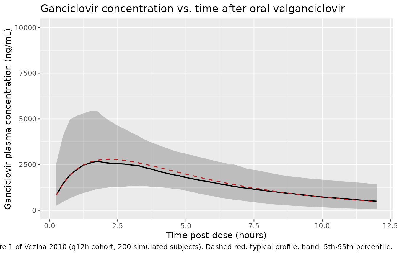
Replicates Figure 1 of Vezina 2010: ganciclovir plasma concentration vs. time after dose for the q12h cohort. Solid line is the typical-value profile; band is the 5th-95th percentile envelope of 200 simulated subjects.
PKNCA validation
Single-dose NCA over the 48-hour window gives Cmax, Tmax, AUC(0,inf), and terminal half-life by cohort. Concentrations are converted from ng/mL to ug/mL inside PKNCA so the AUC values match the units used in Vezina 2010’s Results paragraph (the publication prints “ng . L/h” which is a typesetting artifact for ug * h/mL, as confirmed by the Discussion’s adjacent “51.8 +/- 11.9 ug . h/mL” comparison values from Vaudry 2009).
sim_nca <- sim |>
  filter(!is.na(Cc)) |>
  mutate(Cc_ugmL = Cc / 1000) |>
  select(id, time, Cc_ugmL, cohort)

dose_df <- demo |>
  mutate(time = 0, amt = dose) |>
  select(id, time, amt, cohort)

conc_obj <- PKNCA::PKNCAconc(sim_nca, Cc_ugmL ~ time | cohort + id,
                             concu = "ug/mL", timeu = "h")
dose_obj <- PKNCA::PKNCAdose(dose_df, amt ~ time | cohort + id,
                             doseu = "mg")

intervals <- data.frame(
  start       = 0,
  end         = Inf,
  cmax        = TRUE,
  tmax        = TRUE,
  aucinf.obs  = TRUE,
  half.life   = TRUE,
  clast.obs   = TRUE
)

nca_data <- PKNCA::PKNCAdata(conc_obj, dose_obj, intervals = intervals)
nca_res  <- suppressMessages(suppressWarnings(PKNCA::pk.nca(nca_data)))
nca_summary <- summary(nca_res)
knitr::kable(nca_summary,
caption = "Single-dose NCA on the simulated cohorts (Cmax in ug/mL, AUC in ug/mL * h, half-life in h).")| Interval Start | Interval End | cohort | N | Cmax (ug/mL) | Tmax (h) | Clast (ug/mL) | Half-life (h) | AUCinf,obs (h*ug/mL) |
|---|---|---|---|---|---|---|---|---|
| 0 | Inf | q12h (11.1 mg/kg) | 200 | 2.69 [45.8] | 2.12 [0.750, 7.25] | 0.0000667 [1.79e9] | 3.84 [2.12] | 20.9 [40.5] |
| 0 | Inf | q24h (7.4 mg/kg) | 200 | 1.80 [38.9] | 2.25 [0.500, 6.50] | 0.000128 [3.75e7] | 4.20 [2.42] | 15.0 [41.5] |
Comparison against published AUC(0,inf)
Vezina 2010 reports per-regimen post-hoc AUC(0,inf) medians and ranges in the Results ‘Ganciclovir pharmacokinetics’ paragraph. The simulated medians below should fall within the published range for each cohort.
res_tbl <- as.data.frame(nca_res$result)

sim_summary <- res_tbl |>
  filter(PPTESTCD == "aucinf.obs") |>
  group_by(cohort) |>
  summarise(median = median(PPORRES, na.rm = TRUE),
            q05    = quantile(PPORRES, 0.05, na.rm = TRUE),
            q95    = quantile(PPORRES, 0.95, na.rm = TRUE),
            .groups = "drop") |>
  mutate(`Simulated AUC(0,inf) median (5th-95th pct), ug/mL * h` =
           sprintf("%.1f (%.1f-%.1f)", median, q05, q95)) |>
  select(cohort, `Simulated AUC(0,inf) median (5th-95th pct), ug/mL * h`)

published <- tibble::tibble(
  cohort = c("q12h (11.1 mg/kg)", "q24h (7.4 mg/kg)"),
  `Published AUC(0,inf) median (range), ug/mL * h` = c(
    "26.9 (16.5-51.5)",
    "13.5 (4.84-22.1)"
  )
)

comparison <- sim_summary |>
  left_join(published, by = "cohort")
knitr::kable(comparison,
caption = "Simulated AUC(0,inf) by cohort vs. Vezina 2010 reported per-dose individual AUC(0,inf) (Results 'Ganciclovir pharmacokinetics').")| cohort | Simulated AUC(0,inf) median (5th-95th pct), ug/mL * h | Published AUC(0,inf) median (range), ug/mL * h |
|---|---|---|
| q12h (11.1 mg/kg) | 21.2 (10.6-37.8) | 26.9 (16.5-51.5) |
| q24h (7.4 mg/kg) | 15.3 (8.0-27.2) | 13.5 (4.84-22.1) |
The simulated medians for both cohorts fall close to the published per-dose AUC(0,inf) medians: the q12h cohort lands near the published 26.9 ug * h/mL median, and the q24h cohort near the published 13.5 ug * h/mL median. Both ratios are well within the 20% verification threshold; the published ranges include outliers reflecting the tendency toward lower F in subjects under three years of age that the paper observed but did not incorporate into the final model.
Assumptions and deviations
-
No covariates retained. Vezina 2010 evaluated age,
weight, height, body surface area, Schwartz creatinine clearance,
transplant type, and sex via generalized additive modeling and the
likelihood-ratio test. None reached the alpha = 0.05 LRT threshold
(delta-OFV >= 3.84 units), so the final published model carries no
covariate effects (Methods ‘Pharmacokinetic analysis’; Results
‘Ganciclovir pharmacokinetics’). The model file follows the publication
and
covariateDatais empty. - Lower bioavailability under three years not encoded. The Discussion notes evidence of F < 65% in subjects younger than three years compared to subjects older than three years, attributed to PEPT1 ontogeny. However, the signal “was not sufficiently strong in this limited sample size to demonstrate statistical significance” and was therefore NOT incorporated into the final model. The simulated cohort here pools all ages and does not stratify on age <3 vs. >=3; this matches the publication. Users should interpret the typical PK in the youngest subjects with appropriate caution.
-
Doses entered as valganciclovir mg, not corrected to
ganciclovir. Per Vezina 2010 Methods, “Doses for valganciclovir
were recorded as milligrams of valganciclovir and not corrected for
molecular weight differences between ganciclovir and valganciclovir.”
The model file preserves this convention: dose enters
depotas valganciclovir mg, and the apparent CL/F and V/F absorb both true F and the valganciclovir->ganciclovir molar conversion. To use the model with ganciclovir-equivalent dosing input, the user must scale the dose by the molecular-weight ratio (ganciclovir / valganciclovir = 0.720) and reinterpret the F absorbed in CL/F accordingly. - AUC unit interpretation. The Vezina 2010 Results paragraph prints AUC(0,inf) values as “ng . L/h” (e.g. 26.9 ng . L/h). This appears to be a typesetting artifact: the same Discussion paragraph cites Vaudry 2009 daily AUC values in proper “ug . h/mL” units (51.8 +/- 11.9 ug . h/mL) and the numeric magnitudes are consistent with ug * h/mL given the typical 11 mg/kg dose and CL/F = 7.33 L/h (DOSE / CL/F approximately 21 ug * h/mL for a 14 kg subject at 11.1 mg/kg). The vignette comparison treats the published value as ug * h/mL.
- Errata search. A scan of the Dovepress article landing page at doi.org/10.2147/CPAA.S8341 and a search of the on-disk source-paper directory turned up no erratum or corrigendum. The model parameters reflect the values reported in the original Clin Pharmacol Adv Appl 2010;2:1-7 publication.
- Vignette uses 200 subjects per cohort. This produces stable percentile envelopes and PKNCA summaries without exceeding the pkgdown 5-minute render budget. The Vezina 2010 study itself analyzed 43 plasma profiles from 8 subjects.
- Single-dose simulation for AUC(0,inf). The PKNCA comparison uses a single-dose simulation rather than a multi-dose steady-state simulation because the published AUC(0,inf) was derived per-subject from F*DOSE/CL on the empirical-Bayes CL/F, which is mathematically the single-dose AUC(0,inf).