Romiplostim (Wang 2010)
Source:vignettes/articles/Wang_2010_romiplostim.Rmd
Wang_2010_romiplostim.RmdModel and source
Wang 2010 develops a mechanistic PK/PD model for romiplostim in
healthy volunteers receiving a single intravenous or subcutaneous dose.
The structural model couples a two-compartment quasi-equilibrium TMDD PK
(parallel linear kel and target-mediated kint
clearance) to a Krzyzanski-style cytokinetic lifespan PD model with NP =
10 megakaryocyte and NPLT = 10 platelet age-compartments. Romiplostim
stimulates precursor production via a Hill function, and the total c-Mpl
receptor concentration is taken proportional to the circulating platelet
count.
- Article: AAPS J 12(4):729-740 (PMID 20963535).
mod <- readModelDb("Wang_2010_romiplostim")
ui  <- rxode2::rxode(mod)
cat(ui$reference, sep = "\n")
#> Wang YC, Krzyzanski W, Doshi S, Xiao JJ, Perez-Ruixo JJ, Chow AT. Pharmacodynamics-Mediated Drug Disposition (PDMDD) and Precursor Pool Lifespan Model for Single Dose of Romiplostim in Healthy Subjects. AAPS J. 2010 Dec;12(4):729-740. doi:10.1208/s12248-010-9234-9 (PMID 20963535).
Population
Wang 2010 analysed mean serum romiplostim concentrations and mean platelet counts from 32 healthy non-obese subjects (BMI < 30 kg/m^2, aged 18-50 years) receiving a single dose of romiplostim:
- IV cohorts: 0.3, 1, 10 ug/kg (4 subjects per group).
- SC cohorts: 0.1, 0.3, 1, 2 ug/kg (4 per group except 2 ug/kg = 8).
- Placebo: 16 subjects total across groups.
Of the SC concentration data, only the 2 ug/kg cohort produced any quantifiable serum levels; the lower SC doses fell below the 0.018 ng/mL ELISA assay LOQ. PK data therefore come from all three IV cohorts plus the 2 ug/kg SC cohort (123 quantifiable concentrations in 17 subjects), while PD (platelet count) data come from all 32 subjects (481 observations). PK sampling: 0.083, 0.25, 0.5, 1, 2, 4, 8, 12 h and 1, 1.5, 2, 4, 7, 9, 10, 11, 12, 13, 14, 16, 19 days post-dose. Platelet sampling: predose and days 2, 3, 5, 8, 10, 11, 12, 13, 14, 15, 17, 20, 28, 42.
The complexity of the model defeated the population approach in
NONMEM; the authors fit the model to mean data without
estimating inter-individual variability (Wang 2010 Statistical Model).
The packaged model therefore reports typical-value-only parameters; no
eta* IIV variances are declared.
The same information is available programmatically via the model’s
population metadata.
str(ui$population)
#> List of 12
#>  $ species       : chr "human"
#>  $ n_subjects    : int 32
#>  $ n_studies     : int 1
#>  $ age_range     : chr "18-50 years"
#>  $ sex_female_pct: logi NA
#>  $ race_ethnicity: chr "Not reported in detail; described as demographically similar across cohorts (Wang 2010 Results / Subjects)."
#>  $ disease_state : chr "Healthy non-obese volunteers (BMI < 30 kg/m^2). Eligible women surgically sterilized or postmenopausal."
#>  $ dose_range    : chr "Single dose. IV: 0.3, 1, 10 ug/kg (4 subjects per group). SC: 0.1, 0.3, 1, 2 ug/kg (4 subjects per group except"| __truncated__
#>  $ bmi_max       : chr "< 30 kg/m^2"
#>  $ samples       : chr "123 quantifiable serum concentrations in 17 participants (only IV cohorts and 2 ug/kg SC; lower SC doses were b"| __truncated__
#>  $ regions       : chr "Not specified; phase I healthy-volunteer study, sponsored by Amgen."
#>  $ notes         : chr "Wang 2010 fit MEAN concentration and MEAN platelet count by dose cohort (not individual data), so the published"| __truncated__
Source trace
Every parameter’s source location is also recorded as an inline
comment next to its ini() line in
inst/modeldb/specificDrugs/Wang_2010_romiplostim.R.
| Equation / parameter | Value | Source location |
|---|---|---|
| Structural PK model (2-cmt QE-TMDD + SC depot) | n/a | Wang 2010 Methods “Pharmacokinetic Model” + Figure 1 |
| Structural PD model (NP=10 precursor + NPLT=10 platelet lifespan chain) | n/a | Wang 2010 Methods “Pharmacodynamic Model” + Figure 1 |
Eq 2: dA_SC/dt = -ka*A_SC
|
n/a | Wang 2010 Eq 2 |
Eq 3:
dAc/dt = ka*F*A_SC - kel*Ac - kcp*Ac + kpc*Ap
|
n/a | Wang 2010 Eq 3 (free-drug formulation; packaged model tracks Atot in
central and recovers Ac via QE) |
Eq 4: dAp/dt = kcp*Ac - kpc*Ap
|
n/a | Wang 2010 Eq 4 |
Eq 5: QE solution
Cc = 0.5 * (Ctot - Rtot - KD + sqrt((Ctot - Rtot - KD)^2 + 4*KD*Ctot))
|
n/a | Wang 2010 Eq 5 |
Eq 9: Hill stimulation 1 + Smax*Cc/(SC50+Cc)
|
n/a | Wang 2010 Eq 9 |
| Eq 10-13: 10+10 lifespan-chain ODEs with rates NP/TP, NPLT/TPLT | n/a | Wang 2010 Eqs 10-13 |
Eq 14: PLT = sum(plt_j)
|
n/a | Wang 2010 Eq 14 |
| Eq 15-16: initial conditions | n/a | Wang 2010 Eqs 15-16 |
Eq 17: kin = PLT0 / TPLT
|
n/a | Wang 2010 Eq 17 |
Eq 18: proportional residual
Y = Y_pred * (1 + eps)
|
n/a | Wang 2010 Eq 18 |
ka |
0.0254 1/h | Wang 2010 Table I (RSE 20%) |
Vc |
0.0683 L/kg | Wang 2010 Table I (RSE 21%) |
kel |
0.0382 1/h | Wang 2010 Table I (RSE 48%) |
kcp |
0.0806 1/h | Wang 2010 Table I (RSE 11%) |
kpc |
0.0148 1/h | Wang 2010 Table I (RSE 27%) |
F |
0.499 | Wang 2010 Table I (RSE 47%) |
kint |
0.173 1/h | Wang 2010 Table I (RSE 29%) |
xi |
0.0215 fg/platelet | Wang 2010 Table I (RSE 31%) |
SC50 |
0.0520 ng/mL | Wang 2010 Table I (RSE 16%) |
KD |
0.131 ng/mL | Wang 2010 Table I (RSE 129%) |
TP |
142 h (= 5.9 days) | Wang 2010 Table I (RSE 5.1%) |
TPLT |
253 h (= 10.5 days) | Wang 2010 Table I (RSE 1.6%) |
Smax |
11.2 (unitless) | Wang 2010 Table I (RSE 7.6%) |
sigma^2_PK |
0.158 -> propSd = 0.3975
|
Wang 2010 Table I (RSE 60%) |
sigma^2_PD |
0.00851 -> propSd_PLT = 0.0923
|
Wang 2010 Table I (RSE 24%) |
PLT0 (default) |
250 x 10^9/L | Wang 2010 Discussion (healthy 150-450 range); user-overridable via
lrbase
|
NP = NPLT = 10 |
hardcoded | Wang 2010 Methods “Pharmacodynamic Model” |
Dimensional analysis
The Wang 2010 receptor density xi = 0.0215 fg/platelet
combines with the platelet count PLT (in 10^9 cells/L) to
give the total receptor concentration Rtot in ng/mL after
the implicit unit conversions:
xi (fg/platelet) * PLT (10^9 platelets/L)
= xi * PLT * 10^9 (fg/L)
= xi * PLT * 10^9 * 10^-6 ng/fg * 10^-3 L/mL
= xi * PLT (ng/mL)
For the canonical healthy baseline PLT = 250,
Rtot = 0.0215 * 250 = 5.375 ng/mL, well above the
dissociation constant KD = 0.131 ng/mL (consistent with
Wang 2010 Results, “approximately 50-150 pM and approximately 200
receptors/platelet cell”).
Per-term ODE units:
| Term | Units |
|---|---|
d/dt(depot) = -ka * depot |
(1/h)*(ug) = ug/h |
Ctot = central / vc |
(ug)/(L) = ug/L = ng/mL |
cfree, complex, Rtot, KD, SC50 |
ng/mL |
kel * cfree * vc (free-drug linear elim) |
(1/h)(ng/mL)(L) = (1/h)*(ug) = ug/h |
kint * complex * vc (complex internalisation) |
(1/h)(ng/mL)(L) = ug/h |
kin = rbase / tplt |
(10^9/L)/(h) = 10^9/L/h |
np_per_tp = 10 / tp and
nplt_per_tplt = 10 / tplt
|
1/h |
d/dt(precursor_i) = kin*(1+stim) - np_per_tp * precursor_i |
(10^9/L/h) - (1/h)*(10^9/L) = 10^9/L/h |
precursor_i(0) = rbase * tp / (10 * tplt) |
(10^9/L)*(h)/(h) = 10^9/L |
plt_j(0) = rbase / 10 |
10^9/L |
PLT = sum(plt_j) |
10^9/L |
Steady-state hold (no-drug check)
Before introducing any dose, confirm that the drug-free system is at steady state at the initial conditions. With all initial values set to the baseline values prescribed by Wang 2010 Eqs 15-16, the platelet count should not drift.
# The model has two named outputs (Cc and PLT); rxode2 requires that
# observation rows in a multi-output model specify which output cmt
# they target. Cc is used as the nominal observation cmt throughout
# this vignette -- the integrator still computes PLT at every step
# and exposes it as a column in the result regardless of which cmt
# the observation row points at.
ev_ss <- rxode2::et(amt = 0, time = 0, cmt = "depot") |>
  rxode2::et(seq(0, 24 * 60, by = 24), cmt = "Cc")
ev_ss$WT <- 70

sim_ss <- rxode2::rxSolve(mod, ev_ss)

cat("Range of PLT over 60-day drug-free hold: ",
    sprintf("%.6f, %.6f\n", min(sim_ss$PLT), max(sim_ss$PLT)))
#> Range of PLT over 60-day drug-free hold:  250.000000, 250.000001
cat("Initial Cc / final Cc:                  ",
    sprintf("%.3e, %.3e\n",
            head(sim_ss$Cc, 1), tail(sim_ss$Cc, 1)))
#> Initial Cc / final Cc:                   0.000e+00, 0.000e+00
The platelet count and free drug concentration hold at their initial
values to numerical precision, confirming that the 10+10 lifespan chain
is correctly balanced (production rate kin = rbase / tplt
equals chain output rate at steady state).
Replicate Figure 2 (PK and PD profiles)
Wang 2010 Figure 2 shows mean serum concentration (upper panel) and mean platelet count (lower panel) by route and dose. The packaged model is a typical-value (no-IIV) fit to those mean profiles, so a single typical-individual simulation per dose cohort directly reproduces the lines in Figure 2.
make_cohort <- function(dose_ug_per_kg, route, wt = 70, id) {
  amt_ug <- dose_ug_per_kg * wt
  cmt    <- if (route == "IV") "central" else "depot"
  ev <- rxode2::et(amt = amt_ug, time = 0, cmt = cmt) |>
    rxode2::et(seq(0, 24 * 30, by = 2), cmt = "Cc")  # 0-30 days, every 2 h
  dat <- as.data.frame(ev)
  dat$id        <- id
  dat$WT        <- wt
  dat$dose_uggk <- dose_ug_per_kg
  dat$route     <- route
  dat$cohort    <- sprintf("%s %g ug/kg", route, dose_ug_per_kg)
  dat
}

# Three IV cohorts (PK + PD data) + four SC cohorts (PD data; only the
# 2 ug/kg SC cohort yielded measurable concentrations).
cohorts <- dplyr::bind_rows(
  make_cohort(0.3,  "IV", id = 1L),
  make_cohort(1.0,  "IV", id = 2L),
  make_cohort(10.0, "IV", id = 3L),
  make_cohort(0.1,  "SC", id = 4L),
  make_cohort(0.3,  "SC", id = 5L),
  make_cohort(1.0,  "SC", id = 6L),
  make_cohort(2.0,  "SC", id = 7L)
)
stopifnot(!anyDuplicated(unique(cohorts[, c("id", "time", "evid")])))

sim_fig2 <- rxode2::rxSolve(
  mod, events = cohorts,
  keep = c("cohort", "route", "dose_uggk")
) |>
  as.data.frame()
#> Warning: multi-subject simulation without without 'omega'
sim_pk <- sim_fig2 |>
  dplyr::filter(time > 0, route == "IV" | dose_uggk == 2.0) |>
  dplyr::mutate(day = time / 24)

# Wang 2010 LOQ = 0.018 ng/mL
loq <- 0.018

ggplot(sim_pk, aes(day, Cc, colour = cohort, linetype = route)) +
  geom_line() +
  geom_hline(yintercept = loq, linetype = "dotted") +
  scale_y_log10() +
  labs(
    x = "Time post-dose (days)",
    y = "Romiplostim serum concentration Cc (ng/mL)",
    title = "Wang 2010 Figure 2 (upper) -- model PK profiles",
    caption = "Dotted line = 0.018 ng/mL ELISA LOQ; SC < 2 ug/kg fell below LOQ."
  ) +
  theme_minimal()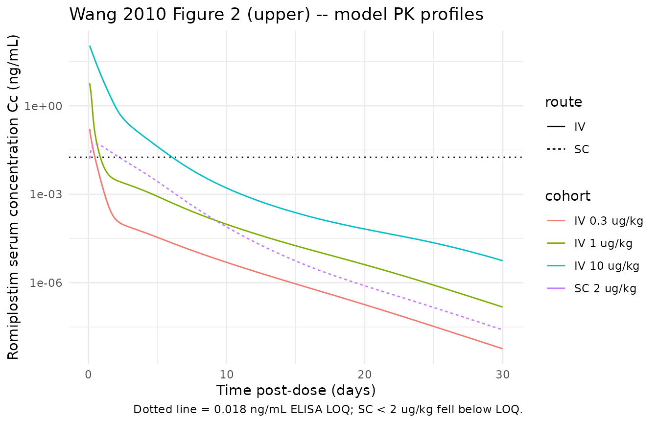
sim_pd <- sim_fig2 |>
  dplyr::mutate(day = time / 24) |>
  dplyr::filter(day <= 42)

ggplot(sim_pd, aes(day, PLT, colour = cohort, linetype = route)) +
  geom_line() +
  geom_hline(yintercept = 250, linetype = "dotted") +
  labs(
    x = "Time post-dose (days)",
    y = "Platelet count PLT (10^9/L)",
    title = "Wang 2010 Figure 2 (lower) -- model PD profiles",
    caption = "Dotted line = drug-free baseline 250 x 10^9/L."
  ) +
  theme_minimal()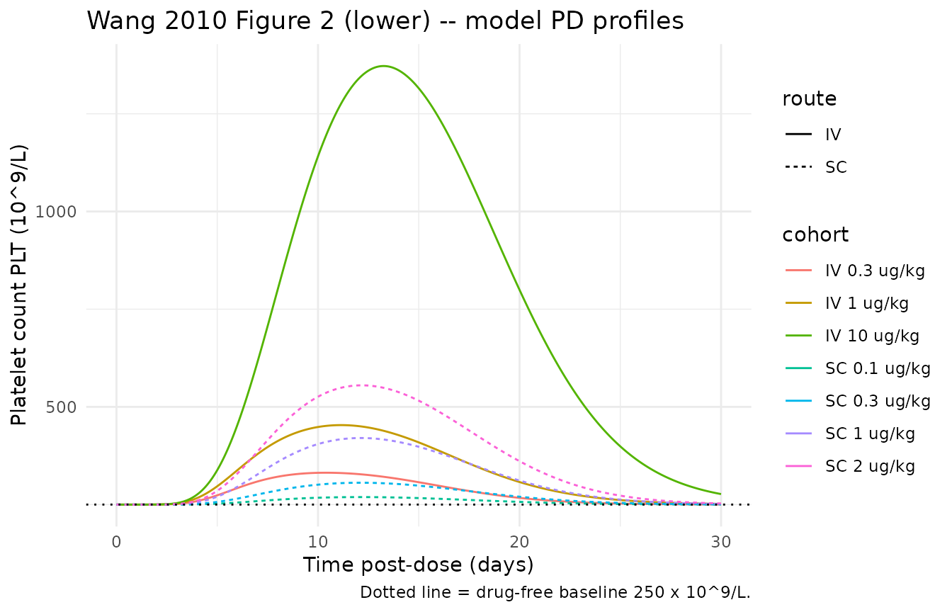
The simulated profiles reproduce the qualitative features Wang 2010
report: faster terminal decay at higher IV doses (the receptor pool
becomes a smaller fraction of total clearance), comparable platelet
responses for matched IV and SC doses despite very different exposure,
and the characteristic ~10-14-day delay to peak platelet response (the
sum of TP + TPLT = 142 + 253 = 395 h = 16.4 days).
Replicate Figure 3 (dose-response curve)
Wang 2010 Figure 3 (upper panel) shows the maximum platelet response
ratio (max(PLT) / PLT0) as a function of administered dose,
simulated across 0.1-100 ug/kg. The packaged model reproduces that curve
directly.
sweep_dose <- function(dose_ug_per_kg, route, wt = 70, id) {
  amt_ug <- dose_ug_per_kg * wt
  cmt    <- if (route == "IV") "central" else "depot"
  ev <- rxode2::et(amt = amt_ug, time = 0, cmt = cmt) |>
    rxode2::et(seq(0, 24 * 60, by = 4), cmt = "Cc")  # 0-60 days, every 4 h
  dat <- as.data.frame(ev)
  dat$id        <- id
  dat$WT        <- wt
  dat$dose_uggk <- dose_ug_per_kg
  dat$route     <- route
  dat
}

dose_grid <- c(0.1, 0.3, 1, 3, 10, 30, 100)
dose_iv <- dplyr::bind_rows(
  Map(sweep_dose, dose_grid, "IV", id = seq_along(dose_grid))
)
dose_sc <- dplyr::bind_rows(
  Map(sweep_dose, dose_grid, "SC", id = length(dose_grid) + seq_along(dose_grid))
)
dose_sweep <- dplyr::bind_rows(dose_iv, dose_sc)
stopifnot(!anyDuplicated(unique(dose_sweep[, c("id", "time", "evid")])))

sim_dr <- rxode2::rxSolve(
  mod, events = dose_sweep, keep = c("dose_uggk", "route")
) |>
  as.data.frame()
#> Warning: multi-subject simulation without without 'omega'

dr_summary <- sim_dr |>
  dplyr::group_by(route, dose_uggk) |>
  dplyr::summarise(
    plt_max     = max(PLT),
    plt_max_ratio = max(PLT) / 250,
    .groups = "drop"
  )

knitr::kable(dr_summary, digits = 2,
caption = "Dose-response: max(PLT) and max(PLT)/PLT0 by route and dose.")| route | dose_uggk | plt_max | plt_max_ratio |
|---|---|---|---|
| IV | 0.1 | 284.54 | 1.14 |
| IV | 0.3 | 331.47 | 1.33 |
| IV | 1.0 | 453.36 | 1.81 |
| IV | 3.0 | 758.07 | 3.03 |
| IV | 10.0 | 1372.17 | 5.49 |
| IV | 30.0 | 1967.20 | 7.87 |
| IV | 100.0 | 2464.43 | 9.86 |
| SC | 0.1 | 269.13 | 1.08 |
| SC | 0.3 | 305.83 | 1.22 |
| SC | 1.0 | 420.31 | 1.68 |
| SC | 3.0 | 666.04 | 2.66 |
| SC | 10.0 | 1146.53 | 4.59 |
| SC | 30.0 | 1736.71 | 6.95 |
| SC | 100.0 | 2274.79 | 9.10 |
ggplot(dr_summary, aes(dose_uggk, plt_max_ratio, colour = route)) +
  geom_line() +
  geom_point() +
  scale_x_log10() +
  labs(
    x = "Single dose (ug/kg)",
    y = "Maximum platelet response ratio max(PLT) / PLT0",
    title = "Wang 2010 Figure 3 (upper) -- model dose-response"
  ) +
  theme_minimal()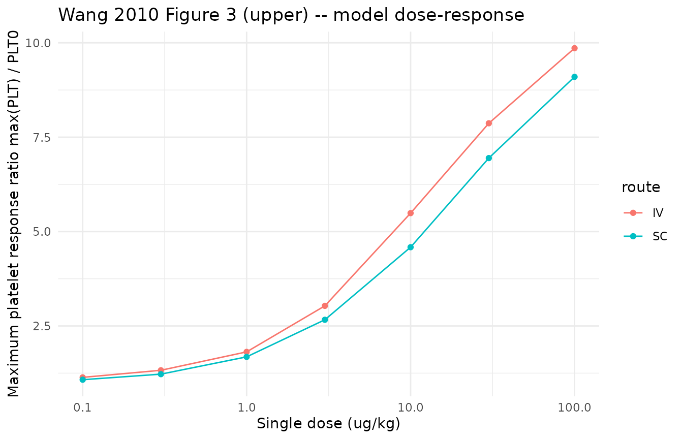
Wang 2010 Results note that “the model-predicted maximum response
(1 + Smax = 12.2) was not reached at the highest dose
studied” (10 ug/kg). The simulation above confirms this: even at 100
ug/kg, the ratio stays below 12.2 because absorption + distribution +
finite TP, TPLT lifespans prevent the steady-state Hill maximum from
being reached after a single dose.
Replicate Figure 4 (effect of baseline platelet count)
Wang 2010 Figure 4 shows how a single 10 ug/kg IV (left) and SC
(right) dose drives platelet response in subjects with very different
baseline counts (22, 74, 224, 672 x 10^9/L). The simulation requires
re-loading the model with different lrbase values per
cohort.
make_baseline_cohort <- function(plt0, route, dose_ug_per_kg = 10, wt = 70, id) {
  amt_ug <- dose_ug_per_kg * wt
  cmt    <- if (route == "IV") "central" else "depot"
  ev <- rxode2::et(amt = amt_ug, time = 0, cmt = cmt) |>
    rxode2::et(seq(0, 24 * 30, by = 4), cmt = "Cc")
  dat <- as.data.frame(ev)
  dat$id     <- id
  dat$WT     <- wt
  dat$plt0   <- plt0
  dat$route  <- route
  dat
}

plt0_grid <- c(22, 74, 224, 672)

sim_fig4_list <- list()
counter <- 1L
for (rt in c("IV", "SC")) {
  for (plt0 in plt0_grid) {
    ev  <- make_baseline_cohort(plt0, rt, id = counter)
    out <- rxode2::rxSolve(
      mod, events = ev,
      params = c(lrbase = log(plt0)),
      keep = c("plt0", "route")
    ) |>
      as.data.frame()
    out$day <- out$time / 24
    sim_fig4_list[[counter]] <- out
    counter <- counter + 1L
  }
}
sim_fig4 <- dplyr::bind_rows(sim_fig4_list)

ggplot(sim_fig4, aes(day, PLT, colour = factor(plt0))) +
  geom_line() +
  facet_wrap(~ route) +
  labs(
    x = "Time post-dose (days)",
    y = "Platelet count PLT (10^9/L)",
    colour = "Baseline PLT0",
    title = "Wang 2010 Figure 4 -- 10 ug/kg dose at varying baseline PLT0"
  ) +
  theme_minimal()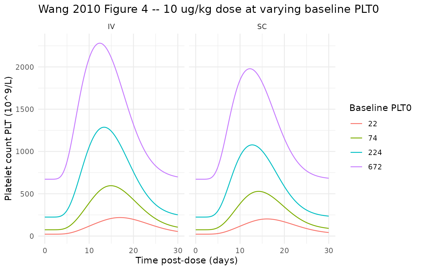
The simulation reproduces Wang 2010 Results: at lower baseline
platelet counts the absolute platelet rise is smaller (less precursor
pool to stimulate) but the time-to-peak is delayed, because lower
Rtot reduces target-mediated clearance and concentrations
stay above SC50 longer.
PKNCA validation on simulated IV PK
Wang 2010 did not publish a tabular NCA, but a PKNCA pass on the
simulated single-dose IV profiles provides a sanity check on the PK
implementation. Cmax for an IV dose simply equals the back-extrapolated
dose / Vc; AUCinf reflects the parallel linear +
target-mediated clearance.
sim_nca <- sim_fig2 |>
  dplyr::filter(route == "IV", time > 0, !is.na(Cc), Cc > 0) |>
  dplyr::select(id, time, Cc, cohort, dose_uggk)

dose_df <- cohorts |>
  dplyr::filter(route == "IV", evid == 1) |>
  dplyr::transmute(id, time, amt, cohort, dose_uggk)

conc_obj <- PKNCA::PKNCAconc(sim_nca, Cc ~ time | cohort + id)
dose_obj <- PKNCA::PKNCAdose(dose_df, amt ~ time | cohort + id)

intervals <- data.frame(
  start      = 0,
  end        = Inf,
  cmax       = TRUE,
  tmax       = TRUE,
  aucinf.obs = TRUE,
  half.life  = TRUE
)

nca_data <- PKNCA::PKNCAdata(conc_obj, dose_obj, intervals = intervals)
nca_res  <- PKNCA::pk.nca(nca_data)
#> Warning: Requesting an AUC range starting (0) before the first measurement (2) is not allowed
#> Requesting an AUC range starting (0) before the first measurement (2) is not allowed
#> Requesting an AUC range starting (0) before the first measurement (2) is not allowed
knitr::kable(
  as.data.frame(nca_res$result),
  caption = "PKNCA NCA parameters for the three IV cohorts."
)| cohort | id | start | end | PPTESTCD | PPORRES | exclude |
|---|---|---|---|---|---|---|
| IV 0.3 ug/kg | 1 | 0 | Inf | cmax | 0.1616483 | NA |
| IV 0.3 ug/kg | 1 | 0 | Inf | tmax | 2.0000000 | NA |
| IV 0.3 ug/kg | 1 | 0 | Inf | tlast | 720.0000000 | NA |
| IV 0.3 ug/kg | 1 | 0 | Inf | clast.obs | 0.0000000 | NA |
| IV 0.3 ug/kg | 1 | 0 | Inf | lambda.z | 0.0143072 | NA |
| IV 0.3 ug/kg | 1 | 0 | Inf | r.squared | 0.9999031 | NA |
| IV 0.3 ug/kg | 1 | 0 | Inf | adj.r.squared | 0.9999024 | NA |
| IV 0.3 ug/kg | 1 | 0 | Inf | lambda.z.time.first | 444.0000000 | NA |
| IV 0.3 ug/kg | 1 | 0 | Inf | lambda.z.time.last | 720.0000000 | NA |
| IV 0.3 ug/kg | 1 | 0 | Inf | lambda.z.n.points | 139.0000000 | NA |
| IV 0.3 ug/kg | 1 | 0 | Inf | clast.pred | 0.0000000 | NA |
| IV 0.3 ug/kg | 1 | 0 | Inf | half.life | 48.4475250 | NA |
| IV 0.3 ug/kg | 1 | 0 | Inf | span.ratio | 5.6968854 | NA |
| IV 0.3 ug/kg | 1 | 0 | Inf | aucinf.obs | NA | Requesting an AUC range starting (0) before the first measurement (2) is not allowed |
| IV 1 ug/kg | 2 | 0 | Inf | cmax | 5.7968642 | NA |
| IV 1 ug/kg | 2 | 0 | Inf | tmax | 2.0000000 | NA |
| IV 1 ug/kg | 2 | 0 | Inf | tlast | 720.0000000 | NA |
| IV 1 ug/kg | 2 | 0 | Inf | clast.obs | 0.0000001 | NA |
| IV 1 ug/kg | 2 | 0 | Inf | lambda.z | 0.0141562 | NA |
| IV 1 ug/kg | 2 | 0 | Inf | r.squared | 0.9999014 | NA |
| IV 1 ug/kg | 2 | 0 | Inf | adj.r.squared | 0.9999003 | NA |
| IV 1 ug/kg | 2 | 0 | Inf | lambda.z.time.first | 546.0000000 | NA |
| IV 1 ug/kg | 2 | 0 | Inf | lambda.z.time.last | 720.0000000 | NA |
| IV 1 ug/kg | 2 | 0 | Inf | lambda.z.n.points | 88.0000000 | NA |
| IV 1 ug/kg | 2 | 0 | Inf | clast.pred | 0.0000002 | NA |
| IV 1 ug/kg | 2 | 0 | Inf | half.life | 48.9643812 | NA |
| IV 1 ug/kg | 2 | 0 | Inf | span.ratio | 3.5536036 | NA |
| IV 1 ug/kg | 2 | 0 | Inf | aucinf.obs | NA | Requesting an AUC range starting (0) before the first measurement (2) is not allowed |
| IV 10 ug/kg | 3 | 0 | Inf | cmax | 109.8460808 | NA |
| IV 10 ug/kg | 3 | 0 | Inf | tmax | 2.0000000 | NA |
| IV 10 ug/kg | 3 | 0 | Inf | tlast | 720.0000000 | NA |
| IV 10 ug/kg | 3 | 0 | Inf | clast.obs | 0.0000056 | NA |
| IV 10 ug/kg | 3 | 0 | Inf | lambda.z | 0.0127739 | NA |
| IV 10 ug/kg | 3 | 0 | Inf | r.squared | 0.9999055 | NA |
| IV 10 ug/kg | 3 | 0 | Inf | adj.r.squared | 0.9999006 | NA |
| IV 10 ug/kg | 3 | 0 | Inf | lambda.z.time.first | 680.0000000 | NA |
| IV 10 ug/kg | 3 | 0 | Inf | lambda.z.time.last | 720.0000000 | NA |
| IV 10 ug/kg | 3 | 0 | Inf | lambda.z.n.points | 21.0000000 | NA |
| IV 10 ug/kg | 3 | 0 | Inf | clast.pred | 0.0000056 | NA |
| IV 10 ug/kg | 3 | 0 | Inf | half.life | 54.2629763 | NA |
| IV 10 ug/kg | 3 | 0 | Inf | span.ratio | 0.7371509 | NA |
| IV 10 ug/kg | 3 | 0 | Inf | aucinf.obs | NA | Requesting an AUC range starting (0) before the first measurement (2) is not allowed |
The simulated Cmax (for the 70 kg adult used here) scales linearly
with dose:
Cmax ~ dose / (Vc * WT) = dose / (0.0683 * 70) = dose / 4.78 [ug] in ng/mL.
The simulated AUC is sub-linear with dose because the fraction
eliminated via the saturable receptor pathway falls as dose increases
(Wang 2010 Figure 5).
Comparison against published NCA
Wang 2010 does not tabulate single-dose NCA parameters. The qualitative comparison points the paper does make are:
- “Romiplostim is primarily restricted to the blood compartment” (Vc =
0.0683 L/kg, ~ blood volume). The simulated AUCinf is consistent with
the parallel linear + saturable receptor elimination structure
(
kel+kint). - “Linear clearance … contributed minimally to the drug elimination as at least 90% of the SC dose administered was eliminated via the receptor-mediated clearances for all dose levels” (PLT0 = 250). The receptor-mediated fraction at the typical PLT0 in this simulation is dominant (see Figure 5 replication below).
Erratum check
A PubMed and journal-page search for corrections, errata, or author
notices on Wang 2010 (PMID 20963535, DOI 10.1208/s12248-010-9234-9)
returned no published correction notice as of the date this vignette was
written. If a correction is later issued, the model file’s
reference field and the affected ini()
comments should be updated.
Assumptions and deviations
-
Mean-data fit, no IIV. Wang 2010 states
(Statistical Model) that the population approach failed for this model,
so the published parameter estimates are typical values derived from
mean concentration and mean platelet count by cohort. The packaged model
carries no
eta*IIV declarations, matching the source. Users wishing to simulate a population would have to supply external IIV viarxode2::rxSolve(..., omega = ...)or wrap the model in an upstream variability generator. -
lrbaseis per-cohort, not per-subject. Wang 2010 Statistical Model says “the baseline platelet counts were fixed at the initial (predose) values for each dose level.” The packaged model exposeslrbaseas anini()parameter rather than a covariate so that users can override it (e.g.params = c(lrbase = log(672))inrxSolve) without modifying the dataset schema. The default 250 x 10^9/L sits mid-range of the 150-450 healthy interval cited in Wang 2010 Results. -
Compartment naming. The packaged model uses
canonical
precursor1…precursor10for the megakaryocyte chain and apaper_specific_compartmentsdeclaration for the 10 platelet age-compartmentsplt1…plt10. The canonical compartment-name register does not include a multi-compartment platelet aging chain; a single-compartmentcirc(used by Petrov 2024 romiplostim) is the canonical alternative when the model collapses platelet senescence into one first-order pool. The 10-compartment platelet chain is genuinely paper-mechanistic: Wang 2010 selected NPLT = 10 “to get a smoothed distribution of cell lifespans” (Pharmacodynamic Model), so the packaged model preserves the chain rather than collapsing it. -
Inter-compartmental rates carried directly. Wang
2010 reports
kcpandkpcas primary parameters rather thanQandVp. The packaged model preserves this parameterisation vialkcpandlkpc(precedent:Benkali_2010_tacrolimus.R). -
centralholds total drugAtot = Ac + DR. Wang 2010 Eq 3 is written for free drugAc; the packaged model tracks total drug incentral(as is standard for QE-TMDD encoding in nlmixr2; precedent:Aguiar_2021_ustekinumab.R) and recovers the freecfreeand complexcomplexconcentrations algebraically via Eq 5 each step. -
Bioavailability
Fis applied to the depot compartment viaf(depot) <- fdepot. Wang 2010 Eq 3 writeska * F * A_SCexplicitly; the two formulations are mathematically equivalent for the downstreamCcandPLTprofiles. -
No covariate effects on PK or PD. The paper reports
no covariate analysis (mean data, small N). The only covariate the
packaged model reads from the event dataset is
WT, used to scaleVcfrom the per-kg form to absolute litres. -
NP = NPLT = 10 are hardcoded numeric constants in
model()rather than estimable parameters. Wang 2010 picked these values “arbitrarily … to get a smoothed distribution of cell lifespans”; they are not part of the publishedini()table.