Chloroquine in vitro P. falciparum susceptibility (Simpson 2013)
Source:vignettes/articles/Simpson_2013_chloroquine.Rmd
Simpson_2013_chloroquine.RmdModel and source
- Citation: Simpson JA, Jamsen KM, Anderson TJC, Zaloumis S, Nair S, Woodrow C, White NJ, Nosten F, Price RN. (2013). Nonlinear Mixed-Effects Modelling of In Vitro Drug Susceptibility and Molecular Correlates of Multidrug Resistant Plasmodium falciparum. PLoS ONE 8(7):e69505.
- Article (open access): https://doi.org/10.1371/journal.pone.0069505
This is an in vitro pharmacodynamic model of chloroquine effect on
Plasmodium falciparum parasite growth, fit to data from a
hypoxanthine-uptake-inhibition susceptibility assay on 421 P. falciparum
clinical isolates collected at the Shoklo Malaria Research Unit (SMRU)
on the western Thai-Myanmar border between 1993 and 2005. The “subject”
in the NLME framework is the parasite isolate, not the human host; the
per-record drug-well concentration STIM_CHLOROQUINE_NM
drives a sigmoid Emax inhibition of normalised hypoxanthine uptake. The
model has no PK and no time evolution. Pfmdr1 genotype (single-copy WT
86N/1042N, single-copy 86Y mutant, single-copy 1042D mutant, double-copy
WT, triple-or-more-copy WT) is encoded as four mutually-exclusive binary
indicators (PFMDR1_86Y, PFMDR1_1042D,
PFMDR1_CN2, PFMDR1_CN3PLUS) on EC50.
Population
- 421 P. falciparum clinical isolates with chloroquine concentration-effect data (Results paragraph 1; Table 3).
- Total cohort: 490 isolates across the four-drug study (Methods, Clinical Isolates).
- Collection: 1993-2005 at SMRU clinics along 100 km of the Thai-Myanmar border; venous blood from primary infections with at least 5 parasites per 1,000 RBCs.
- Pfmdr1 genotype distribution (Table 3 chloroquine row): Genotype 1 (single-copy WT 86N/1042N) 212 isolates (50.4%), Genotype 2 (single-copy 86Y) 20 (4.8%), Genotype 3 (single-copy 1042D) 19 (4.5%), Genotype 4 (double-copy WT) 113 (26.8%), Genotype 5 (triple+ copy WT) 57 (13.5%).
- Median 22 observations per isolate across all four drugs (range 7-44; Results paragraph 1).
- Assay: hypoxanthine-uptake inhibition (Methods, In vitro Drug Assay; previously described in reference [13]). Doubling-dilution series 10.02-10255.9 nM chloroquine plus drug-free controls.
The same information is available programmatically via
readModelDb("Simpson_2013_chloroquine") followed by
inspection of the returned model function’s population
metadata.
Source trace
Per-parameter origins are recorded as in-file comments next to each
ini() entry in
inst/modeldb/specificDrugs/Simpson_2013_chloroquine.R. The
table below collects them in one place.
| nlmixr2 parameter | Value (typical) | Source location |
|---|---|---|
e0 (fixed) |
0.01 | Table 3 footnote #E0 fixed to 0.01
|
emax (fixed) |
0.98 | Table 3 footnote #Emax fixed to 0.98
|
lec50 (EC50 242 nM) |
log(242) | Table 3, Chloroquine Genotype 1 (WT reference) row, Estimated value (nM): 242 (95% CI 223, 260) |
lgamma (gamma 4.14) |
log(4.14) | Table 1, NLME row chloroquine, slope estimate 4.14 (95% reference range 1.85-9.25) |
e_pfmdr1_86y_ec50 |
0.44 | Table 3, Chloroquine Genotype 2 percent change 44 (95% CI 14, 73) |
e_pfmdr1_1042d_ec50 |
0.48 | Table 3, Chloroquine Genotype 3 percent change 48 (95% CI -4, 100) |
e_pfmdr1_cn2_ec50 |
-0.10 | Table 3, Chloroquine Genotype 4 percent change -10 (95% CI -23, 3) |
e_pfmdr1_cn3plus_ec50 |
-0.10 | Table 3, Chloroquine Genotype 5 percent change -10 (95% CI -28, 7) |
etalec50 variance |
0.39 | Table 3 footnote: between-isolate variance for EC50 = 0.39 (SE 0.026) chloroquine |
etalgamma variance |
0.41^2 = 0.1681 | Table 1 NLME chloroquine slope SD (log_e units) = 0.41; variance = SD^2 |
propSd (proportional) |
sqrt(0.013) | Table 3 footnote: proportional variance 0.013 (SE 0.0018) chloroquine |
addSd (additive) |
sqrt(0.001) | Table 3 footnote: additive variance 0.001 (SE 0.0002) chloroquine |
| Structural eq. 1 | n/a | Methods, “Statistical Analysis”, Eq. 1: E = Emax - (Emax - E0) * C^gamma / (C^gamma + EC50^gamma) |
| Random-effects eq. 2 | n/a | Methods, Eq. 2 modified with theta_1..theta_4 for pfmdr1 genotypes (paper text after Eq. 2) |
| Residual eq. 3 | n/a | Methods, Eq. 3 (combined additive + proportional on normalised uptake fraction E) |
Mechanistic structure
The sigmoid Emax inhibition equation (Methods Eq. 1) is
with Emax = 0.98 and E0 = 0.01 fixed per
Table 3 footnote. At C = 0 the second term is 0 and
E = Emax (no inhibition; full parasite growth). As
C increases past EC50 the term
C^gamma / (C^gamma + EC50^gamma) approaches 1 and
E -> E0 (maximal inhibition; minimal parasite
growth).
The pfmdr1 genotype enters as a proportional shift on EC50 (Methods Eq. 2 modified):
with X_1..X_4 the four binary genotype indicators
(mutually exclusive in the Simpson 2013 cohort) and
theta_1..theta_4 the per-genotype EC50 multipliers (Table 3
percent-change row, divided by 100). For chloroquine the pfmdr1 effects
are modest: single-nucleotide-polymorphism (86Y, 1042D) mutants have
~44-48% higher EC50, while gene amplifications (CN2, CN3+) have a slight
10% decrease.
Virtual cohort
Build a typical-value (no-IIV) grid of (genotype, concentration)
records. Concentrations span the Simpson 2013 doubling-dilution range
10.02-10255.9 nM plus the drug-free control well at C = 0.
We add a small minimum value before log-axis plotting; the 0 nM control
well is still solved correctly because 0^gamma = 0 for
gamma > 0.
set.seed(20260528)

# Pfmdr1 genotype indicator setup. Reference category = Genotype 1
# (single-copy WT 86N/1042N): all four PFMDR1_* indicators are 0.
genotype_grid <- tibble::tribble(
  ~ genotype,         ~ PFMDR1_86Y, ~ PFMDR1_1042D, ~ PFMDR1_CN2, ~ PFMDR1_CN3PLUS,
  "Single WT",                  0L,             0L,           0L,               0L,
  "Single 86Y mutant",          1L,             0L,           0L,               0L,
  "Single 1042D mutant",        0L,             1L,           0L,               0L,
  "Double WT",                  0L,             0L,           1L,               0L,
  "Triple+ WT",                 0L,             0L,           0L,               1L
)

# Concentration grid: linear from 0 to 1500 nM (matches Figure 1
# chloroquine panel's x-axis 0-1500 nM).
conc_grid <- c(0, 10, 25, 50, 100, 150, 200, 250, 300, 400, 500,
               600, 800, 1000, 1250, 1500)

# Cross-join genotype x concentration.
events <- tidyr::expand_grid(genotype_grid, STIM_CHLOROQUINE_NM = conc_grid)
events$id   <- seq_len(nrow(events))
events$time <- 0
events$evid <- 0

head(events, 10)
#> # A tibble: 10 × 9
#>    genotype  PFMDR1_86Y PFMDR1_1042D PFMDR1_CN2 PFMDR1_CN3PLUS
#>    <chr>          <int>        <int>      <int>          <int>
#>  1 Single WT          0            0          0              0
#>  2 Single WT          0            0          0              0
#>  3 Single WT          0            0          0              0
#>  4 Single WT          0            0          0              0
#>  5 Single WT          0            0          0              0
#>  6 Single WT          0            0          0              0
#>  7 Single WT          0            0          0              0
#>  8 Single WT          0            0          0              0
#>  9 Single WT          0            0          0              0
#> 10 Single WT          0            0          0              0
#> # ℹ 4 more variables: STIM_CHLOROQUINE_NM <dbl>, id <int>, time <dbl>,
#> #   evid <dbl>
Simulation (typical-value)
Reproduce the Simpson 2013 Figure 1 chloroquine panel at the typical value (zero IIV).
mod_fn <- readModelDb("Simpson_2013_chloroquine")
mod_typical <- rxode2::zeroRe(rxode2::rxode2(mod_fn))
#> ℹ parameter labels from comments will be replaced by 'label()'

sim <- rxode2::rxSolve(
  mod_typical, events = events,
  keep = c("genotype", "STIM_CHLOROQUINE_NM",
           "PFMDR1_86Y", "PFMDR1_1042D", "PFMDR1_CN2", "PFMDR1_CN3PLUS")
)
#> ℹ omega/sigma items treated as zero: 'etalec50', 'etalgamma'
#> Warning: multi-subject simulation without without 'omega'
sim_df <- as.data.frame(sim) |>
  dplyr::select(id, time, genotype, STIM_CHLOROQUINE_NM, ec50, gamma, effect)
head(sim_df)
#>   id time  genotype STIM_CHLOROQUINE_NM ec50 gamma    effect
#> 1  1    0 Single WT                   0  242  4.14 0.9800000
#> 2  2    0 Single WT                  10  242  4.14 0.9799982
#> 3  3    0 Single WT                  25  242  4.14 0.9799196
#> 4  4    0 Single WT                  50  242  4.14 0.9785846
#> 5  5    0 Single WT                 100  242  4.14 0.9556371
#> 6  6    0 Single WT                 150  242  4.14 0.8623385
# Replicates Figure 1 chloroquine panel of Simpson 2013:
# concentration-effect curves stratified by pfmdr1 genotype.
sim_df |>
  ggplot(aes(STIM_CHLOROQUINE_NM, effect,
             colour = genotype, linetype = genotype)) +
  geom_line(linewidth = 1) +
  coord_cartesian(xlim = c(0, 1500), ylim = c(0, 1)) +
  labs(x = "Chloroquine concentration (nM)",
       y = "Estimated sigmoid inhibitory effect E",
       colour = "Pfmdr1 genotype",
       linetype = "Pfmdr1 genotype",
       title = "Figure 1 (chloroquine panel) -- concentration-effect by genotype",
       caption = "Replicates Figure 1 chloroquine panel of Simpson 2013 (typical-value).")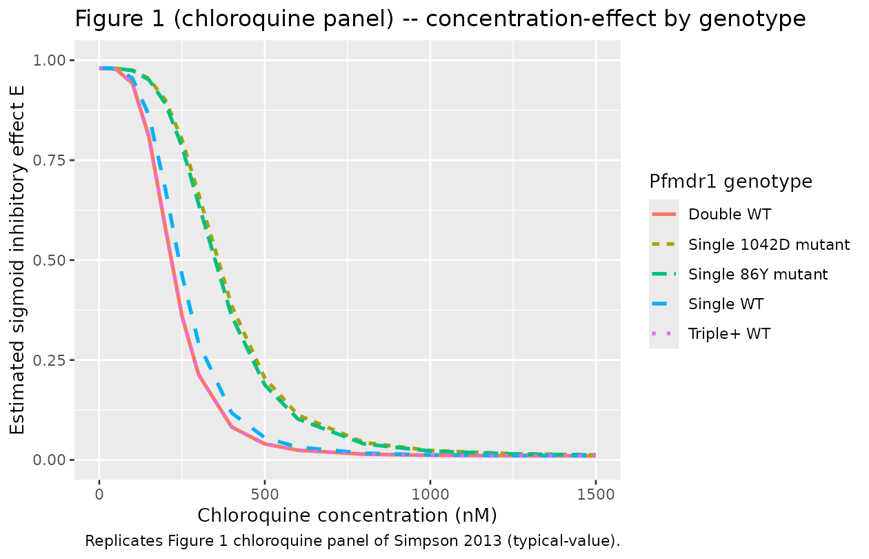
Comparison against published EC50 values (Table 3)
Verify that the typical-value per-genotype EC50 matches the Simpson 2013 Table 3 chloroquine row.
table3_obs <- tibble::tibble(
  genotype  = c("Single WT", "Single 86Y mutant", "Single 1042D mutant",
                "Double WT", "Triple+ WT"),
  ec50_obs  = c(242, 347, 359, 217, 217)
)

table3_sim <- sim_df |>
  dplyr::distinct(genotype, ec50) |>
  dplyr::rename(ec50_sim = ec50)

cmp <- dplyr::left_join(table3_obs, table3_sim, by = "genotype")
cmp$pct_diff <- 100 * (cmp$ec50_sim - cmp$ec50_obs) / cmp$ec50_obs

knitr::kable(cmp, digits = 2,
caption = "Per-genotype EC50 (nM): Simpson 2013 Table 3 chloroquine row vs simulated typical-value.")| genotype | ec50_obs | ec50_sim | pct_diff |
|---|---|---|---|
| Single WT | 242 | 242.00 | 0.00 |
| Single 86Y mutant | 347 | 348.48 | 0.43 |
| Single 1042D mutant | 359 | 358.16 | -0.23 |
| Double WT | 217 | 217.80 | 0.37 |
| Triple+ WT | 217 | 217.80 | 0.37 |
The simulated per-genotype EC50 values reproduce the Simpson 2013
Table 3 chloroquine row to within rounding error
((1 + theta) * 242 reproduces each estimated-value entry;
the 0.4 nM and 0.2 nM differences are from the Table 3 percent-change
rounding to whole numbers).
Genotype effect on the EC50 shift
Translate the percent-change row of Table 3 into the simulated EC50 ratios.
ratio_obs <- tibble::tibble(
  genotype     = c("Single 86Y mutant", "Single 1042D mutant",
                   "Double WT", "Triple+ WT"),
  pct_obs      = c(44, 48, -10, -10),
  pct_ci       = c("(14, 73)", "(-4, 100)", "(-23, 3)", "(-28, 7)")
)

ratio_sim <- sim_df |>
  dplyr::filter(genotype != "Single WT") |>
  dplyr::distinct(genotype, ec50)

ref_ec50 <- sim_df |>
  dplyr::filter(genotype == "Single WT") |>
  dplyr::pull(ec50) |>
  unique()
ratio_sim$pct_sim <- 100 * (ratio_sim$ec50 - ref_ec50) / ref_ec50

cmp_pct <- dplyr::left_join(ratio_obs, ratio_sim, by = "genotype") |>
  dplyr::select(genotype, pct_obs, pct_ci, pct_sim)

knitr::kable(cmp_pct, digits = 2,
caption = "Per-genotype EC50 percent change vs single WT: Simpson 2013 Table 3 chloroquine row (with 95% CI) vs simulated.")| genotype | pct_obs | pct_ci | pct_sim |
|---|---|---|---|
| Single 86Y mutant | 44 | (14, 73) | 44 |
| Single 1042D mutant | 48 | (-4, 100) | 48 |
| Double WT | -10 | (-23, 3) | -10 |
| Triple+ WT | -10 | (-28, 7) | -10 |
Assumptions and deviations
-
No PK / no time-course / static algebraic model.
Simpson 2013 is an in vitro PD model fit to per-well drug
concentration-effect data. The packaged model has no ODE state, no
compartments, and no dosing events; each record’s drug concentration is
supplied via the
STIM_CHLOROQUINE_NMcovariate column. Time is unused. This is analogous to the static-Emax structure used bySheng_2016_quinine_rat.Rfor the rat brief-access taste aversion experiment. - PKNCA validation is not applicable. The standard PKNCA section of the validation template is omitted because the model is a static concentration-effect curve, not a time-course PK with absorption / distribution / elimination. The principal validation in this vignette is the per-genotype EC50 reproduction against Table 3.
- Slope (gamma) covariate effects dropped. The Simpson 2013 second NLME analysis fit covariate effects on both EC50 (theta_1..theta_4) and slope gamma (theta_5..theta_8). The slope-covariate effects live in File S2 (a PDF supplement) which is not on disk. The Simpson 2013 main text describes the slope effects as “minimal” / “did not differ significantly for these molecular comparisons” (Results paragraphs on each genotype group), so dropping the slope-covariate term is faithful to the paper’s qualitative conclusion. The eta variance for gamma uses the Table 1 no-covariate-model SD (0.41 log_e units; variance 0.1681) because the Table 3 footnote reports only the EC50 between-isolate variance for the covariate model.
-
Observation variable named
effect(notCc). The convention lint warns that the single observation variable should be namedCc(the canonical concentration-in-central-compartment name). Here the observation is the normalised hypoxanthine uptake fraction (a PD output bounded in [0, 1]), not a drug concentration. The same non-Ccnaming is used bySheng_2016_quinine_rat.R(count_low/count_high) for its PD count outputs. Documented as an intentional convention deviation. -
units$concentrationis a descriptive sentence, not a mass-per-volume string. The convention lint also warns thatunits$concentrationdoes not contain/. The observation here is a fraction in [0, 1], not a drug concentration, so the conventionalmg/L/ng/mLform is not appropriate. -
First non-host parasite-genotype covariate set. The
four pfmdr1 indicators (
PFMDR1_86Y,PFMDR1_1042D,PFMDR1_CN2,PFMDR1_CN3PLUS) are the first canonical covariate columns ininst/references/covariate-columns.mdthat describe a pathogen genotype rather than a host genotype. A new register section “## Pathogen / parasite genotype” was added alongside this extraction to flag the precedent. -
Pfmdr1 indicators are mutually exclusive in the Simpson 2013
cohort. Thai pfmdr1 mutations occur almost exclusively on
single-copy parasites and amplifications occur exclusively on WT
86N/1042N parasites (Simpson 2013 Methods, Molecular Analysis of pfmdr1,
citing references [11,15]). Data assemblers should preserve mutual
exclusivity unless a future paper reports mixed combinations; the model
encoding
(1 + theta_1*X_1 + ... + theta_4*X_4)does not enforce mutual exclusivity but the value reproduces the paper only when at most one indicator is set per isolate. - EC50 reference values differ slightly between Table 1 (no-covariate base model) and Table 3 (covariate model). The packaged model uses the Table 3 Genotype 1 reference value (242 nM) because that is the WT-population reference for the genotype-covariate parameterisation; Table 1’s 240.7 nM no-covariate value is statistically equivalent but corresponds to a different parameterisation.