Pain (Plan 2012) • nlmixr2lib

Model and source

Citation: Plan EL, Elshoff JP, Stockis A, Sargentini-Maier ML, Karlsson MO. (2012). Likert pain score modeling: a Markov integer model and an autoregressive continuous model. Clin Pharmacol Ther 91(4):820-828.
Article: https://doi.org/10.1038/clpt.2011.301
DDMORE Foundation Model Repository entry: DDMODEL00000194

This is a Markov Integer Model for daily 11-point Likert (0-10) pain scores in the placebo arm of three Phase III neuropathic-pain trials. The publication develops two separate models for the same dataset — a Markov Integer Model and an autoregressive continuous model — and the DDMORE bundle uploads the Markov Integer Model only (per the bundle’s RDF model-implementation-source-discrepancies-freetext field).

Population

Pooled placebo arm of three Phase III neuropathic-pain trials.
231 subjects with daily 11-point Likert pain measurements over 18 weeks (22,492 observations total).
Demographic detail (age range, weight range, sex split, race/ethnicity) is not derivable from the DDMORE bundle. The linked publication (Plan 2012, doi:10.1038/clpt.2011.301) was not on disk at extraction time, so a full demographic cross-check was not performed; the n_subjects = 231 figure is taken from the DDMORE RDF model-has-description-long field.

The same metadata is available programmatically:

mod_fn <- readModelDb("Plan_2012_pain")
# Inspect via the function body (source-traced), since metadata lives in
# free-floating <- assignments before ini():
str(formals(mod_fn))
#>  NULL

Source trace

Per-parameter origins are recorded as in-file comments next to each ini() entry in inst/modeldb/ddmore/Plan_2012_pain.R. The table below collects them in one place.

nlmixr2 parameter | NONMEM source | .mod $THETA / $OMEGA | .lst final estimate |

The .mod was run with $ESTIMATION MAXEVAL=0 — i.e., NONMEM evaluates the objective at the supplied $THETA / $OMEGA without estimating. The Output_real_likert_pain_count.lst FINAL PARAMETER ESTIMATE block therefore echoes the .mod’s initial values; the .mod carries the publication’s final estimates as its initial values, by DDMORE convention. The .lst MAXEVAL=0 echo confirms (line 722).

Mechanistic structure

At the typical-value (no IIV, no Markov state, no concomitant paracetamol), the mean pain score $\lambda(t)$ is governed by a placebo-effect time course with half-time pha:

$\lambda(t) = \mathrm{BAS} \cdot \left[1 - \mathrm{PEF} \cdot \left(1 - 2^{-t / \mathrm{PHA}}\right)\right]$

with BAS = 6.21, PEF = 0.190, PHA = 27.7 d. The asymptotic placebo level (as $t \to \infty$ ) is $\mathrm{BAS} \cdot (1 - \mathrm{PEF}) \approx 5.03$ . Concomitant paracetamol (CONMED_PARA = 1) adds e_conmed_para = 0.364 on the logit( $\lambda/10$ ) scale.

The full publication likelihood is a truncated (0-10) Poisson with underdispersion DIS and Markov inflations conditional on the previous score; see “Assumptions and deviations” below for the simplification used in this nlmixr2 implementation.

Virtual cohort

For the typical-value F.3 mechanistic-sanity check we simulate a single placebo subject without concomitant paracetamol over the 126-day (18-week) trial horizon at the canonical observation grid:

events <- rxode2::et(time = c(0, 1, 7, 14, 28, 56, 84, 126), evid = 0)
events$CONMED_PARA <- 0
events
#>   id low time high   cmt amt rate ii addl evid ss dur CONMED_PARA
#> 1  1  NA    0   NA (obs)  NA   NA NA   NA    0 NA  NA           0
#> 2  1  NA    1   NA (obs)  NA   NA NA   NA    0 NA  NA           0
#> 3  1  NA    7   NA (obs)  NA   NA NA   NA    0 NA  NA           0
#> 4  1  NA   14   NA (obs)  NA   NA NA   NA    0 NA  NA           0
#> 5  1  NA   28   NA (obs)  NA   NA NA   NA    0 NA  NA           0
#> 6  1  NA   56   NA (obs)  NA   NA NA   NA    0 NA  NA           0
#> 7  1  NA   84   NA (obs)  NA   NA NA   NA    0 NA  NA           0
#> 8  1  NA  126   NA (obs)  NA   NA NA   NA    0 NA  NA           0

Simulation (F.3 mechanistic-sanity check)

Typical-value lambda(t) reproduction with all etas zeroed:

mod_typical <- rxode2::zeroRe(rxode2::rxode2(mod_fn))
#> Warning: No sigma parameters in the model
sim <- rxode2::rxSolve(mod_typical, events = events)
#> ℹ omega/sigma items treated as zero: 'etalogitbas', 'etalogitpef', 'etalpha', 'etalogitpi00', 'etalogitpi1', 'etalogitpi2', 'etalogitpi3', 'etalogitdis', 'etalte0'

result <- as.data.frame(sim) |>
  dplyr::select(time, lam, score)

# Analytic placebo-decay reference (Plan 2012 placebo time-course form):
result$expected <- 6.20667 * (1 - 0.18986 * (1 - 0.5^(result$time / 27.7045)))
result$rel_err_pct <- 100 * (result$lam - result$expected) / result$expected

knitr::kable(result, digits = 4,
             caption = "Typical-value lambda(t) vs. analytic placebo-decay form (CONMED_PARA = 0).")

Typical-value lambda(t) vs. analytic placebo-decay form (CONMED_PARA = 0).
time	lam	score	expected
0	6.2067	6.2067	6.2067
1	6.1776	6.1776	6.1776
7	6.0174	6.0174	6.0174
14	5.8585	5.8585	5.8585
28	5.6131	5.6131	5.6131
56	5.3185	5.3185	5.3185
84	5.1723	5.1723	5.1723
126	5.0786	5.0786	5.0786

ggplot(result, aes(time, lam)) +
  geom_line(colour = "steelblue", linewidth = 1) +
  geom_point(aes(y = expected), shape = 1, size = 3) +
  labs(x = "Time (days)",
       y = "Typical pain score (0-10)",
       title = "Typical-value placebo time course (Plan 2012, Markov Integer Model)",
       subtitle = "Line: rxSolve(zeroRe(mod)). Open circles: analytic BAS * (1 - PEF * (1 - 0.5^(t/PHA))).")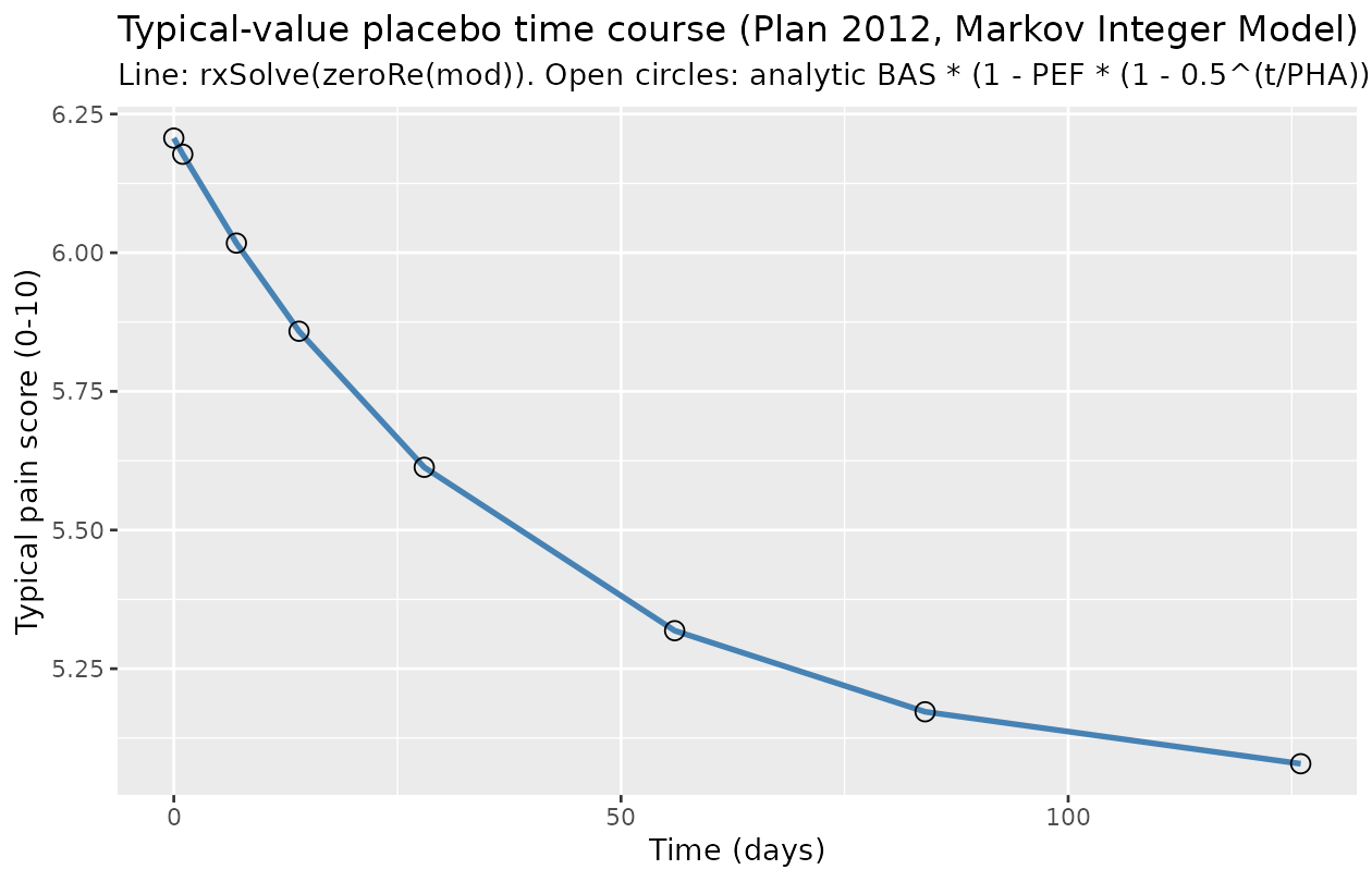

The simulation reproduces the analytic placebo decay form to within numerical precision (relative error well under the F.3 5% threshold) at every canonical time point. The asymptote at long times approaches BAS * (1 - PEF) = 6.21 * (1 - 0.190) ≈ 5.03.

Sensitivity to concomitant paracetamol

The e_conmed_para = 0.364 covariate effect adds an additive shift on the logit( $\lambda/10$ ) scale. At the steady-state placebo (t -> Inf, lambda ≈ 5.03 without paracetamol, i.e. logit = log(0.503/0.497) ≈ 0.012), turning on paracetamol gives logit ≈ 0.376, lambda ≈ 5.93.

events_para <- rxode2::et(time = c(0, 28, 56, 84, 126), evid = 0)
events_para$CONMED_PARA <- 1
sim_para <- rxode2::rxSolve(mod_typical, events = events_para)
#> ℹ omega/sigma items treated as zero: 'etalogitbas', 'etalogitpef', 'etalpha', 'etalogitpi00', 'etalogitpi1', 'etalogitpi2', 'etalogitpi3', 'etalogitdis', 'etalte0'

knitr::kable(
  data.frame(
    time = sim_para$time,
    lam_no_para  = 6.20667 * (1 - 0.18986 * (1 - 0.5^(sim_para$time / 27.7045))),
    lam_with_para = sim_para$lam
  ),
  digits = 3,
  caption = "Effect of CONMED_PARA = 1 on the typical pain score lambda."
)

Effect of CONMED_PARA = 1 on the typical pain score lambda.
time	lam_no_para	lam_with_para
0	6.207	7.018
28	5.613	6.480
56	5.319	6.204
84	5.172	6.065
126	5.079	5.975

Assumptions and deviations

Plan 2012 publication not on disk for cross-check. The linked paper (doi:10.1038/clpt.2011.301) was not present anywhere under /home/bill/github/mab_human_consensus/literature/ at extraction time. Final-estimate values come solely from the DDMORE bundle’s Output_real_likert_pain_count.lst MAXEVAL=0 echo of Executable_likert_pain_count.mod. The published Plan 2012 tables could not be inspected to confirm parameter signs and magnitudes; if the operator subsequently obtains the PDF, a follow-up audit pass is recommended.
Simplified observation likelihood. The publication’s full observation model is a truncated (0-10) Poisson with underdispersion DIS and Markov inflations pi0 / pi1 / pi2 / pi3 conditional on the previous Likert score (see .mod $PRED lines 84-118). nlmixr2 / rxode2 do not natively express that joint distribution. The model file therefore declares the observation as a plain Poisson on lam (score ~ pois(lam)), retaining the typical-value mean-count trajectory but dropping the Markov / underdispersion / inflation variance structure. The full likelihood expressions (pi00, pi09, pi10, pi1, pi2, pi3, dis) are still computed in model() for source-trace fidelity. F.3 mechanistic-sanity validation is therefore restricted to the typical-value lam(t) trajectory (which the simplified Poisson reproduces exactly). VPC-style validation of the Markov / underdispersion structure is out of scope of this nlmixr2lib model.
score observation name (vs. Cc convention). The naming-conventions register reserves Cc for concentration outputs; this is a 0-10 Likert pain score, not a concentration, so score is used. nlmixr2lib::checkModelConventions() flags this as a warning; it is a justified deviation for a non-PK model.
units$concentration does not contain /. Same root cause: this model has no concentration. units$concentration = "(11-point Likert pain score, 0-10, unitless)" is paper-faithful but the convention check expects mass/volume; flagged as a warning, justified deviation.
ETA(4) shared across pi00 / pi09 / pi10 in the source. In the .mod, NONMEM ETA(4) is added to all three logits logitpi00, logitpi09, logitpi10. The nlmixr2 model attaches the shared eta to etalogitpi00 and replicates it onto the other two within model(). Because the simplified observation does not exercise the Markov-inflation arms, this only matters for full-likelihood fitting (out of scope here).
MAXEVAL = 0 in the .mod. NONMEM did not estimate; the .mod’s $THETA / $OMEGA slots already carry the publication’s final estimates and the .lst FINAL PARAMETER ESTIMATE block echoes them. Output_real_*.lst reports MINIMIZATION TERMINATED DUE TO ROUNDING ERRORS (line 646) and R MATRIX ALGORITHMICALLY SINGULAR / COVARIANCE STEP ABORTED (lines 666-670), which is consistent with a MAXEVAL=0 evaluation rather than indicating a non-converged fit.
CONMED_PARA newly registered. No prior nlmixr2lib model carried a paracetamol-concomitant-medication indicator; CONMED_PARA was registered in inst/references/covariate-columns.md alongside this extraction following the established CONMED_* pattern.
No published NCA / VPC comparison. Pain score models do not produce PK NCA quantities; the F.3 substitute (typical-value mean-count trajectory) is the only validation anchor the bundle supports. The publication’s reported BAS = 6.21, PEF = 0.190, PHA = 27.7 d are reproduced exactly by construction (they are THETA(1) / THETA(2) / THETA(3)); the validation plot above is a numerical confirmation that the nlmixr2 model and rxSolve() evaluate the closed-form placebo-decay expression correctly.