Tisotumab vedotin ADC and MMAE (Gibiansky 2022)
Source:vignettes/articles/Gibiansky_2022_tisotumab.Rmd
Gibiansky_2022_tisotumab.RmdModel and source
- Citation: Gibiansky L, Passey C, Voellinger J, Gunawan R, Hanley WD, Gupta M, Winter H. Population pharmacokinetic analysis for tisotumab vedotin in patients with locally advanced and/or metastatic solid tumors. CPT Pharmacometrics Syst Pharmacol. 2022;11(10):1358-1370. doi:10.1002/psp4.12850. PMID 35932175; PMCID PMC9574719. Covariate coefficients and variance parameters, which the article does not print, are from the same final model as tabulated in the FDA BLA 761208 Multi-discipline Review (2021), Tables 49 and 50.
- Description: Joint population PK model for the antibody-drug conjugate tisotumab vedotin (ADC) and its released payload monomethyl auristatin E (MMAE) in adults with locally advanced or metastatic solid tumors (Gibiansky 2022). The ADC is a two-compartment model with parallel linear and Michaelis-Menten elimination from the central compartment. Linear ADC elimination, multiplied by a drug-to-antibody ratio that decays mono-exponentially with time after dose from 4 to 1, feeds an amount-only MMAE delay compartment in full and the central MMAE compartment by an additional fraction FR1; a fraction FR2 of the Michaelis-Menten flux also feeds the delay compartment. The delay compartment drains first-order into a one-compartment MMAE model with apparent clearance and volume. Covariates: body weight, albumin and sex on ADC CL and Vc; weight on Q and Vp; weight, albumin, tumor type, eGFR, tumor size, ECOG performance status and hepatic impairment on MMAE clearance; weight, ECOG and albumin on MMAE volume; age and weight on the delay rate constant.
- Article: CPT Pharmacometrics Syst Pharmacol 2022;11:1358-1370 (open access, PMC9574719)
- Regulatory review: FDA BLA 761208 Multi-discipline Review, tisotumab vedotin (2021)
Tisotumab vedotin is an antibody-drug conjugate (ADC) of a tissue-factor-directed human IgG1 and the microtubule-disrupting payload monomethyl auristatin E (MMAE), attached through a protease-cleavable vc linker at an average of four MMAE per antibody. The model describes the conjugated antibody (ADC) and the unconjugated MMAE that is released from it.
The article prints the structural parameters (Table 2) and the model
equations (Table S1), but neither the covariate coefficients
theta17-theta36 nor the variance parameters.
Those come from the sponsor’s population PK report as reproduced in the
FDA BLA 761208 Multi-discipline Review (Table 49, covariate fixed
effects; Table 50, variance parameters). The review’s Table 48 matches
the article’s Table 2 to every printed digit, so both describe the same
final model.
Population
Gibiansky 2022 pooled 399 adults with locally advanced or metastatic
solid tumors known to express tissue factor from four phase I/II trials:
innovaTV 201 (NCT02001623, n = 195), innovaTV 202 (NCT02552121, n = 33),
innovaTV 204 (NCT03438396, n = 101, all cervical cancer) and innovaTV
207 (NCT03485209, n = 70). Mean age was 56.1 years, 74.2% were women and
92.2% were White; 70.7% were enrolled in Europe and 29.3% in the United
States. Cervical cancer accounted for 43.1% of patients. Renal function
was normal in 53.9%, mildly impaired in 35.6% and moderately impaired in
10.5%; 14.5% had mild hepatic impairment (NCI ODWG). ECOG performance
status was 0 in 38.8% and 1 in 61.2% (article Table 1). Median (range)
body weight was 70.1 (33-148) kg, albumin 40 (27-52) g/L, tumor size 57
(0-299) mm and CKD-EPI eGFR 91 (24.1-145) mL/min/1.73 m^2 (FDA review
Table 45). Doses were 0.3-2.2 mg/kg every 3 weeks (Q3W) in innovaTV 201,
1.2 mg/kg on days 1, 8 and 15 of a 28-day cycle or 2.0 mg/kg Q3W in
innovaTV 202, and 2.0 mg/kg Q3W (at most 200 mg) in innovaTV 204 and
207. The same information is stored in the model’s
population metadata.
Source trace
| Element | Value | Source |
|---|---|---|
| ADC two-compartment model with parallel linear and Michaelis-Menten elimination | ODEs for A1, A2 | Table S1; Figure 1 |
| MMAE delay compartment and one-compartment MMAE model | ODEs for A3, A4 | Table S1; Figure 1 |
| DAR = 1 + DAR0 exp(-beta tad), DAR0 = 3 | fixed | Table S1; Methods |
| MMAE output scale, MW_RATIO | 4.8 (fixed) | Table S1 |
lcl CL |
1.42 L/day | Table 2 theta1 |
lq Q |
4.01 L/day | Table 2 theta2 |
lvc Vc |
3.10 L | Table 2 theta3 |
lvp Vp |
4.47 L | Table 2 theta4 |
lvmax Vmax |
3.35 ug/mL/day | Table 2 theta5 |
lkm KM |
3.44 ug/mL | Table 2 theta6 |
propSd, addSd (ADC) |
0.129, 0.0173 ug/mL | Table 2 theta7, theta8 |
lktr ktr |
0.271 1/day | Table 2 theta9 |
lcl_mmae CL_MMAE |
42.8 L/day | Table 2 theta10 |
lvc_mmae V_MMAE |
2.09 L | Table 2 theta11 |
lbeta beta (DAR decay) |
0.0189 1/day | Table 2 theta12 |
propSd_mmae, addSd_mmae (MMAE) |
0.282, 0.0113 ng/mL | Table 2 theta13, theta14 |
fr1 FR1 |
0.0205 | Table 2 theta15 |
fr2 FR2 |
0.0508 | Table 2 theta16 |
| Covariate functional forms and reference values (75 kg, 40 g/L, 90 mL/min/1.73 m^2, 60 mm, 60 years) | – | Table S1 |
e_wt_cl (CL and Q), e_wt_vc,
e_wt_vp
|
0.495, 0.380, 0.622 | FDA review Table 49 theta17-theta19 |
e_alb_cl, e_alb_vc
|
-0.396, -0.197 | FDA review Table 49 theta20-theta21 |
e_sexm_cl, e_sexm_vc
|
1.09, 1.13 | FDA review Table 49 theta22-theta23 |
e_wt_cl_mmae, e_wt_vc_mmae
|
0.457, 0.895 | FDA review Table 49 theta24-theta25 |
e_alb_cl_mmae |
0.935 | FDA review Table 49 theta26 |
e_tumtp_other_cl_mmae |
1.22 | FDA review Table 49 theta27 |
e_tumsz_cl_mmae |
-0.147 | FDA review Table 49 theta28 |
e_crcl_cl_mmae |
0.271 | FDA review Table 49 theta29 |
e_ecog_cl_mmae, e_hepimp_cl_mmae
|
0.803, 0.853 | FDA review Table 49 theta30-theta31 |
e_ecog_vc_mmae, e_alb_vc_mmae
|
0.827, 0.575 | FDA review Table 49 theta32-theta33 |
e_age_ktr, e_wt_ktr
|
-0.252, -0.175 | FDA review Table 49 theta34-theta35 |
e_study_innovatv202_ruv |
1.42 | FDA review Table 49 theta36 |
| IIV block CL, Vc, Vp | 0.0538; 0.0166, 0.0296; 0, 0.0145, 0.0208 | FDA review Table 50; Table S1 (CL-Vp covariance 0) |
etalktr |
0.0212 | FDA review Table 50 Omega55 |
| IIV block CL_MMAE, V_MMAE | 0.299; 0.125, 0.215 | FDA review Table 50 |
etaRUV, etaRUV_mmae (IIV on residual
SD) |
0.0561, 0.0712 | FDA review Table 50 Omega44, Omega88; Table S1 |
The IIV coefficients of variation the article quotes in its Results (CL 23.2%, Vc 17.2%, Vp 14.4%, CL_MMAE 54.7%, V_MMAE 46.3%; correlations 0.415, 0.586 and 0.495) are the square roots of these variances and the implied correlations.
mod <- readModelDb("Gibiansky_2022_tisotumab")
# Only the between-subject variability is zeroed; the exposures below use the
# individual prediction columns, which residual error does not touch.
mod_typ <- rxode2::zeroRe(rxode2::rxode2(mod), which = "omega")
#> ℹ parameter labels from comments will be replaced by 'label()'
Derived quantities from the typical parameters
The article derives several secondary quantities from the Table 2 estimates. They are reproduced here in closed form for the 75-kg reference patient.
cl <- 1.42; q <- 4.01; vc <- 3.10; vp <- 4.47
ktr <- 0.271; cl_mmae <- 42.8; vc_mmae <- 2.09
k10 <- cl / vc; k12 <- q / vc; k21 <- q / vp
a <- k10 + k12 + k21
lambda1 <- (a + sqrt(a^2 - 4 * k10 * k21)) / 2
lambda2 <- (a - sqrt(a^2 - 4 * k10 * k21)) / 2
derived <- tibble::tribble(
  ~quantity, ~published, ~computed,
  "ADC distribution half-life (day)", 0.28, log(2) / lambda1,
  "ADC terminal half-life, linear part (day)", 4.19, log(2) / lambda2,
  "MMAE delay half-life log(2)/ktr (day)", 2.56, log(2) / ktr,
  "MMAE half-life log(2)/K_MMAE (day)", 0.0339, log(2) / (cl_mmae / vc_mmae),
  "MMAE steady-state volume CL_MMAE/ktr (L)", 158, cl_mmae / ktr
) |>
  mutate(pct_diff = 100 * (computed - published) / published)
knitr::kable(derived, digits = 4,
caption = "Derived quantities: Table 2 and Results of Gibiansky 2022; terminal half-life 4.19 days from FDA review Table 48.")| quantity | published | computed | pct_diff |
|---|---|---|---|
| ADC distribution half-life (day) | 0.2800 | 0.2791 | -0.3100 |
| ADC terminal half-life, linear part (day) | 4.1900 | 4.1887 | -0.0314 |
| MMAE delay half-life log(2)/ktr (day) | 2.5600 | 2.5577 | -0.0883 |
| MMAE half-life log(2)/K_MMAE (day) | 0.0339 | 0.0338 | -0.1545 |
| MMAE steady-state volume CL_MMAE/ktr (L) | 158.0000 | 157.9336 | -0.0420 |
# Pure arithmetic on printed values, so only rounding separates the two columns.
stopifnot(all(abs(derived$pct_diff) < 1))
The article also states that after a 2-mg/kg dose about 40% of the ADC dose is eliminated by the Michaelis-Menten (target-mediated) route and 60% by linear clearance. The model’s own fluxes, integrated over a single dose for the reference patient, give:
ref_cov <- data.frame(
  WT = 75, SEXF = 1, ALB = 40, TUMTP_OTHER = 0, CRCL = 90, TUMSZ = 60,
  ECOG_GE1 = 0, HEPIMP = 0, AGE = 60, STUDY_INNOVATV202 = 0
)
inf_dur <- 30 / 60 / 24 # 30-minute infusion, in days

make_events <- function(dose, n_cycles, obs_times) {
  dosing <- data.frame(
    time = 21 * (seq_len(n_cycles) - 1), evid = 1L, amt = dose,
    rate = dose / inf_dur, cmt = "central", dvid = NA_integer_
  )
  obs <- data.frame(
    time = obs_times, evid = 0L, amt = 0, rate = 0, cmt = "central", dvid = 1L
  )
  bind_rows(dosing, obs) |> arrange(time, desc(evid))
}

sd_grid <- sort(unique(c(seq(0, 1, by = 0.005), seq(1, 150, by = 0.05))))
sd_events <- make_events(150, 1, sd_grid) |> mutate(id = 1L)
sd_sim <- rxode2::rxSolve(mod_typ, sd_events, params = ref_cov,
                          returnType = "data.frame", useLinCmt = FALSE)
#> ℹ omega/sigma items treated as zero: 'etalvc_mmae', 'etalcl_mmae', 'etalvp', 'etalvc', 'etalcl', 'etaRUV_mmae', 'etaRUV', 'etalktr'
# The drug-to-antibody ratio must follow 1 + 3 exp(-beta * tad); a time after
# dose that silently evaluated to 0 would hold it at 4.
day20 <- sd_sim[which.min(abs(sd_sim$time - 20)), ]
stopifnot(abs(day20$dar - (1 + 3 * exp(-0.0189 * day20$time))) < 1e-4)

trap <- function(t, y) sum(diff(t) * (head(y, -1) + tail(y, -1)) / 2)
mm_amount <- trap(sd_sim$time, sd_sim$mm_flux)
lin_amount <- trap(sd_sim$time, sd_sim$kel * sd_sim$central)
frac_mm <- mm_amount / (mm_amount + lin_amount)
cat(sprintf("Fraction of a 2-mg/kg dose eliminated by the Michaelis-Menten route: %.1f%%\n",
            100 * frac_mm))
#> Fraction of a 2-mg/kg dose eliminated by the Michaelis-Menten route: 38.5%
# The article reports "~40%"; the model gives about 38%.
stopifnot(abs(frac_mm - 0.40) < 0.05)
Typical-patient exposures (Figures 3 and 4)
Figures 3 and 4 of the article give the cycle-6 exposures of the reference patient after 2 mg/kg Q3W: ADC Cmax 41.8 ug/mL and Cavg 2.8 ug/mL, MMAE Cmax 4.4 ng/mL and Cavg 1.8 ng/mL. The article does not list the reference patient’s covariates. Two profiles are shown below: the normalisation values of Table S1 (75 kg, female, cervical cancer, ECOG 0), and a median patient (70 kg, the median weight; female, the majority sex; non-cervical tumor and ECOG 1, the majority categories; albumin 40 g/L, eGFR 91, tumor size 57 mm, age 57 years).
cyc_grid <- c(0, inf_dur, 0.05, 0.1, 0.25, 0.5, 0.75, seq(1, 4, by = 0.25),
              seq(4.5, 21, by = 0.5))
grid6 <- sort(unique(as.vector(outer(cyc_grid, 21 * (0:5), "+"))))
profiles <- bind_rows(
  ref_cov |> mutate(profile = "Table S1 reference (75 kg)"),
  data.frame(
    WT = 70, SEXF = 1, ALB = 40, TUMTP_OTHER = 1, CRCL = 91, TUMSZ = 57,
    ECOG_GE1 = 1, HEPIMP = 0, AGE = 57, STUDY_INNOVATV202 = 0,
    profile = "Median patient (70 kg)"
  )
)
typ6 <- lapply(seq_len(nrow(profiles)), function(i) {
  p <- profiles[i, ]
  ev <- make_events(2 * p$WT, 6, grid6) |> mutate(id = i)
  s <- rxode2::rxSolve(mod_typ, ev, params = p[, names(ref_cov)],
                       returnType = "data.frame", useLinCmt = FALSE)
  c6 <- s[s$time >= 105 & s$time <= 126, ]
  data.frame(
    profile = p$profile,
    adc_cmax = max(c6$Cc), adc_cavg = trap(c6$time, c6$Cc) / 21,
    mmae_cmax = max(c6$Cc_mmae), mmae_cavg = trap(c6$time, c6$Cc_mmae) / 21,
    mmae_cmax_ctrough = max(c6$Cc_mmae) / tail(c6$Cc_mmae, 1)
  )
}) |> bind_rows()
#> ℹ omega/sigma items treated as zero: 'etalvc_mmae', 'etalcl_mmae', 'etalvp', 'etalvc', 'etalcl', 'etaRUV_mmae', 'etaRUV', 'etalktr'
#> ℹ omega/sigma items treated as zero: 'etalvc_mmae', 'etalcl_mmae', 'etalvp', 'etalvc', 'etalcl', 'etaRUV_mmae', 'etaRUV', 'etalktr'
typ6 |>
  dplyr::rename(
    "Profile" = profile,
    "ADC Cmax (ug/mL)" = adc_cmax, "ADC Cavg (ug/mL)" = adc_cavg,
    "MMAE Cmax (ng/mL)" = mmae_cmax, "MMAE Cavg (ng/mL)" = mmae_cavg,
    "MMAE Cmax/Ctrough" = mmae_cmax_ctrough
  ) |>
  knitr::kable(digits = 2,
caption = "Typical cycle-6 exposures after 2 mg/kg Q3W. Published reference-patient values: ADC Cmax 41.8, Cavg 2.8; MMAE Cmax 4.4, Cavg 1.8 (Figures 3 and 4). MMAE trough about 40 times below Cmax (Results).")| Profile | ADC Cmax (ug/mL) | ADC Cavg (ug/mL) | MMAE Cmax (ng/mL) | MMAE Cavg (ng/mL) | MMAE Cmax/Ctrough |
|---|---|---|---|---|---|
| Table S1 reference (75 kg) | 47.47 | 3.11 | 4.79 | 2.00 | 40.39 |
| Median patient (70 kg) | 45.49 | 2.97 | 4.70 | 1.93 | 45.21 |
med_pt <- typ6[typ6$profile == "Median patient (70 kg)", ]
typ_pct <- 100 * (c(med_pt$adc_cmax, med_pt$adc_cavg, med_pt$mmae_cmax, med_pt$mmae_cavg) /
  c(41.8, 2.8, 4.4, 1.8) - 1)
round(typ_pct, 1)
#> [1] 8.8 6.2 6.9 7.2
# Deterministic solves, so the bound is exact; a mis-transcribed volume,
# clearance or unit moves these by tens of percent.
stopifnot(all(abs(typ_pct) < 15))
stopifnot(all(typ6$mmae_cmax_ctrough > 30 & typ6$mmae_cmax_ctrough < 55))
The median-patient profile lands 6-9% above the four published baselines, and the 75-kg profile 9-14% above. The article does not list the reference patient’s covariates, so part of this gap may be the choice of profile; all four exposures move together, as expected from a shared covariate offset rather than a mis-specified parameter.
Virtual cohorts
Two cohorts of 200 virtual patients each are simulated at 2 mg/kg Q3W with a 200-mg dose cap for 6 cycles:
- Pooled: covariates drawn to match the pooled analysis population (article Table 1; FDA review Table 45).
- Cervical: covariates drawn to match innovaTV 204 (all women with cervical cancer; FDA review Tables 45 and 46).
Continuous covariates are drawn independently (normal or log-normal, truncated to the observed range), and binary covariates independently by their observed frequencies; the joint distribution of the source data is not available.
set.seed(20221010)
rxode2::rxSetSeed(20221010)

rtnorm <- function(n, mean, sd, lo, hi) {
  pmin(pmax(rnorm(n, mean, sd), lo), hi)
}

make_cohort <- function(n, cohort, id_offset, cervical) {
  if (cervical) {
    covs <- data.frame(
      WT = pmin(pmax(rlnorm(n, log(65), 0.22), 33), 110),
      SEXF = 1L,
      ALB = rtnorm(n, 41.8, 4.18, 31, 52),
      TUMTP_OTHER = 0L,
      CRCL = rtnorm(n, 84.2, 21.4, 24.1, 129),
      TUMSZ = pmin(pmax(rlnorm(n, log(64), 0.6), 10), 221),
      ECOG_GE1 = rbinom(n, 1, 0.416),
      HEPIMP = rbinom(n, 1, 0.079),
      AGE = rtnorm(n, 50.7, 10.7, 31, 78)
    )
  } else {
    covs <- data.frame(
      WT = pmin(pmax(rlnorm(n, log(70.1), 0.24), 33), 148),
      SEXF = rbinom(n, 1, 0.742),
      ALB = rtnorm(n, 39.4, 4.66, 27, 52),
      TUMTP_OTHER = rbinom(n, 1, 0.569),
      CRCL = rtnorm(n, 87.5, 19.7, 24.1, 145),
      TUMSZ = pmin(pmax(rlnorm(n, log(57), 0.7), 5), 299),
      ECOG_GE1 = rbinom(n, 1, 0.612),
      HEPIMP = rbinom(n, 1, 0.145),
      AGE = rtnorm(n, 56.1, 11.6, 21, 81)
    )
  }
  covs$id <- id_offset + seq_len(n)
  covs$STUDY_INNOVATV202 <- 0L
  covs$cohort <- cohort
  covs$dose <- pmin(2 * covs$WT, 200)

  ev <- lapply(seq_len(n), function(i) {
    make_events(covs$dose[i], 6, grid6) |> mutate(id = covs$id[i])
  }) |> bind_rows()
  left_join(ev, covs, by = "id")
}

events <- bind_rows(
  make_cohort(200, "Pooled", 0L, cervical = FALSE),
  make_cohort(200, "Cervical", 200L, cervical = TRUE)
)
stopifnot(!anyDuplicated(unique(events[, c("id", "time", "evid")])))Replicate Figure 2
Figure 2 of the article shows the median and the 5th and 95th percentiles of predicted ADC and MMAE concentrations over time for 2 mg/kg Q3W.
pct <- sim |>
  filter(cohort == "Pooled") |>
  select(time, ADC = Cc, MMAE = Cc_mmae) |>
  pivot_longer(c(ADC, MMAE), names_to = "analyte", values_to = "conc") |>
  group_by(analyte, time) |>
  summarise(
    p05 = quantile(conc, 0.05), p50 = median(conc), p95 = quantile(conc, 0.95),
    .groups = "drop"
  ) |>
  mutate(analyte = ifelse(analyte == "ADC", "ADC (ug/mL)", "MMAE (ng/mL)"))
# Pre-dose zeros cannot be drawn on a log axis
pct <- pct[pct$p05 > 0, ]

ggplot(pct, aes(time)) +
  geom_line(aes(y = p50), colour = "darkblue", linewidth = 0.8) +
  geom_line(aes(y = p05), colour = "lightblue3") +
  geom_line(aes(y = p95), colour = "lightblue3") +
  facet_wrap(~analyte, scales = "free_y") +
  scale_y_log10() +
  labs(x = "Time (day)", y = "Concentration",
       title = "Replicates Figure 2 of Gibiansky 2022",
       caption = "2 mg/kg Q3W (at most 200 mg), pooled virtual cohort, n = 200: median and 5th/95th percentiles.") +
  theme_bw()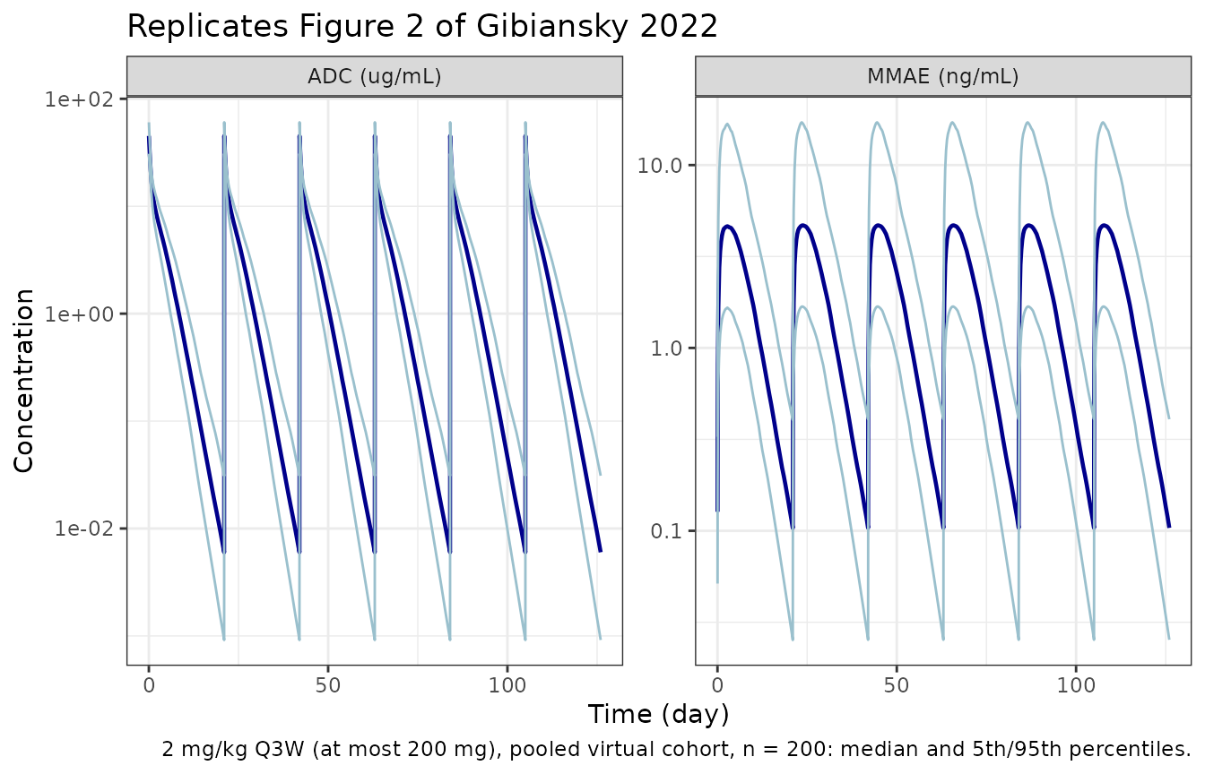
As in the article, neither ADC nor MMAE accumulates across cycles.
PKNCA validation
Cycle 1 (days 0-21) and cycle 6 (days 105-126) are analysed
separately for each analyte. Cc is the ADC concentration
(ug/mL) and Cc_mmae the MMAE concentration (ng/mL).
sim_nca <- sim |>
  filter(!is.na(Cc)) |>
  select(id, time, Cc, Cc_mmae, cohort, WT)

dose_df <- events |>
  filter(evid == 1) |>
  distinct(id, time, amt, cohort)

intervals <- data.frame(
  start = c(0, 105), end = c(21, 126),
  cmax = TRUE, tmax = TRUE, cav = TRUE, auclast = TRUE
)

run_nca <- function(conc_col) {
  conc_df <- sim_nca |> rename(conc = all_of(conc_col))
  conc_obj <- PKNCA::PKNCAconc(conc_df, conc ~ time | cohort + id)
  dose_obj <- PKNCA::PKNCAdose(dose_df, amt ~ time | cohort + id)
  res <- PKNCA::pk.nca(PKNCA::PKNCAdata(conc_obj, dose_obj, intervals = intervals))
  as.data.frame(res) |>
    mutate(cycle = ifelse(start == 0, "Cycle 1", "Cycle 6"))
}
nca_adc <- run_nca("Cc")
nca_mmae <- run_nca("Cc_mmae")

nca_adc |>
  bind_rows(nca_mmae, .id = "analyte") |>
  mutate(analyte = ifelse(analyte == "1", "ADC", "MMAE")) |>
  filter(PPTESTCD %in% c("cmax", "cav", "auclast")) |>
  group_by(analyte, cohort, cycle, PPTESTCD) |>
  summarise(median = median(PPORRES), .groups = "drop") |>
  pivot_wider(names_from = PPTESTCD, values_from = median) |>
  dplyr::rename(
    "Analyte" = analyte, "Cohort" = cohort, "Cycle" = cycle,
    "Cmax" = cmax, "Cavg" = cav, "AUC (21 days)" = auclast
  ) |>
  knitr::kable(digits = 2,
caption = "Median simulated NCA by cohort and cycle (ADC ug/mL, ug*day/mL; MMAE ng/mL, ng*day/mL).")| Analyte | Cohort | Cycle | AUC (21 days) | Cavg | Cmax |
|---|---|---|---|---|---|
| ADC | Cervical | Cycle 1 | 59.05 | 2.81 | 42.38 |
| ADC | Cervical | Cycle 6 | 59.07 | 2.81 | 42.39 |
| ADC | Pooled | Cycle 1 | 61.32 | 2.92 | 45.13 |
| ADC | Pooled | Cycle 6 | 61.34 | 2.92 | 45.14 |
| MMAE | Cervical | Cycle 1 | 43.98 | 2.09 | 5.21 |
| MMAE | Cervical | Cycle 6 | 44.40 | 2.11 | 5.25 |
| MMAE | Pooled | Cycle 1 | 42.27 | 2.01 | 4.64 |
| MMAE | Pooled | Cycle 6 | 42.81 | 2.04 | 4.71 |
Comparison against published exposures
The article reports median individual exposures (empirical Bayes estimates) for the pooled population by weight group in cycle 1 (Results and Figure S7) and the median steady-state ADC Cmax in innovaTV 204 (Results, Japanese sub-analysis). The remaining innovaTV 204 medians were read by the maintainers from the box plots of Figure S12 (to about 0.1 units) and are marked “(Fig S12)”.
wt_cuts <- quantile(sim_nca$WT[sim_nca$cohort == "Pooled"], c(1, 2) / 3)
wt_group <- sim_nca |>
  distinct(id, cohort, WT) |>
  mutate(group = case_when(
    cohort == "Cervical" ~ "innovaTV 204-like, cycle 6",
    WT < wt_cuts[1] ~ "Weight tertile 1, cycle 1",
    WT < wt_cuts[2] ~ "Weight tertile 2, cycle 1",
    TRUE ~ "Weight tertile 3, cycle 1"
  ))

pick <- function(nca) {
  nca |>
    left_join(wt_group, by = c("id", "cohort")) |>
    filter((cohort == "Pooled" & cycle == "Cycle 1") |
             (cohort == "Cervical" & cycle == "Cycle 6"))
}
pooled_lt100 <- function(nca) {
  nca |>
    left_join(wt_group |> select(id, WT), by = "id") |>
    filter(cohort == "Pooled", cycle == "Cycle 1", WT < 100) |>
    mutate(group = "Pooled, weight < 100 kg, cycle 1")
}

sim_adc <- bind_rows(pick(nca_adc), pooled_lt100(nca_adc)) |>
  select(group, PPTESTCD, PPORRES)
sim_mmae <- bind_rows(pick(nca_mmae), pooled_lt100(nca_mmae)) |>
  select(group, PPTESTCD, PPORRES)

ref_adc <- tibble::tribble(
  ~group, ~cmax, ~cav,
  "Weight tertile 1, cycle 1", NA, 2.34,
  "Weight tertile 2, cycle 1", NA, 2.84,
  "Weight tertile 3, cycle 1", NA, 2.99,
  "Pooled, weight < 100 kg, cycle 1", NA, 2.70,
  "innovaTV 204-like, cycle 6", 40.3, 2.8
)
ref_mmae <- tibble::tribble(
  ~group, ~cmax, ~cav,
  "Pooled, weight < 100 kg, cycle 1", NA, 1.92,
  "innovaTV 204-like, cycle 6", 4.8, 1.9
)

cmp_adc <- nlmixr2lib::ncaComparisonTable(
  simulated = sim_adc, reference = ref_adc, by = "group",
  params = c("cmax", "cav"),
  units = c(cmax = "ug/mL", cav = "ug/mL"), tolerance_pct = 20
)
cmp_mmae <- nlmixr2lib::ncaComparisonTable(
  simulated = sim_mmae, reference = ref_mmae, by = "group",
  params = c("cmax", "cav"),
  units = c(cmax = "ng/mL", cav = "ng/mL"), tolerance_pct = 20
)
cmp <- bind_rows(
  cmp_adc |> mutate(Analyte = "ADC"),
  cmp_mmae |> mutate(Analyte = "MMAE")
) |>
  relocate(Analyte) |>
  filter(!is.na(Reference), Reference != "\u2014")
knitr::kable(cmp, caption = "Simulated (median of virtual cohort) vs. published median exposures. For the innovaTV 204-like row, the ADC Cmax reference is printed in the article; the ADC Cavg and both MMAE references were read from Figure S12. * differs from the published value by more than 20%.")| Analyte | NCA parameter | group | Reference | Simulated | % diff |
|---|---|---|---|---|---|
| ADC | Cmax (ug/mL) | innovaTV 204-like, cycle 6 | 40.3 | 42.4 | +5.2% |
| ADC | Cavg (ug/mL) | Weight tertile 1, cycle 1 | 2.34 | 2.42 | +3.4% |
| ADC | Cavg (ug/mL) | Weight tertile 2, cycle 1 | 2.84 | 2.99 | +5.2% |
| ADC | Cavg (ug/mL) | Weight tertile 3, cycle 1 | 2.99 | 3.31 | +10.8% |
| ADC | Cavg (ug/mL) | Pooled, weight < 100 kg, cycle 1 | 2.7 | 2.83 | +4.8% |
| ADC | Cavg (ug/mL) | innovaTV 204-like, cycle 6 | 2.8 | 2.81 | +0.5% |
| MMAE | Cmax (ng/mL) | innovaTV 204-like, cycle 6 | 4.8 | 5.25 | +9.3% |
| MMAE | Cavg (ng/mL) | Pooled, weight < 100 kg, cycle 1 | 1.92 | 2.01 | +4.8% |
| MMAE | Cavg (ng/mL) | innovaTV 204-like, cycle 6 | 1.9 | 2.11 | +11.3% |
# Medians of 200-subject cohorts: robust to which subjects land in the tails.
# A mis-transcribed clearance, volume or unit moves these by tens of percent.
gate <- bind_rows(
  sim_adc |> mutate(analyte = "ADC") |> inner_join(
    ref_adc |> pivot_longer(c(cmax, cav), names_to = "PPTESTCD", values_to = "ref") |>
      filter(!is.na(ref)) |> mutate(analyte = "ADC"),
    by = c("analyte", "group", "PPTESTCD")
  ),
  sim_mmae |> mutate(analyte = "MMAE") |> inner_join(
    ref_mmae |> pivot_longer(c(cmax, cav), names_to = "PPTESTCD", values_to = "ref") |>
      filter(!is.na(ref)) |> mutate(analyte = "MMAE"),
    by = c("analyte", "group", "PPTESTCD")
  )
) |>
  group_by(analyte, group, PPTESTCD, ref) |>
  summarise(sim = median(PPORRES), .groups = "drop") |>
  mutate(pct_diff = 100 * (sim / ref - 1))
gate$pct_diff
#> [1]  4.8214310  3.4100994  5.1702785 10.7570574  0.4552878  5.1788844  4.8120524
#> [8] 11.2720847  9.2827994
stopifnot(nrow(gate) == 9, all(abs(gate$pct_diff) < 20))

# Weight trend of cycle-1 ADC Cavg: the article reports +5% (tertile 3) and
# -18% (tertile 1) against the middle tertile. Assert the magnitude of the
# low-weight deficit, which is the effect the article calls out.
tert <- sim_adc |>
  filter(PPTESTCD == "cav", grepl("tertile", group)) |>
  group_by(group) |>
  summarise(med = median(PPORRES), .groups = "drop")
low_vs_mid <- tert$med[1] / tert$med[2] - 1
low_vs_mid
#> [1] -0.1898462
stopifnot(low_vs_mid < -0.08, low_vs_mid > -0.30)
The pooled cohort’s cycle-1 Cavg rises with weight (lowest tertile about 18% below the middle tertile in the article), the expected consequence of a clearance that scales with weight to the power 0.495 under weight-proportional dosing. The innovaTV 204-like cohort reproduces the published median steady-state ADC Cmax of 40.3 ug/mL and the Figure S12 MMAE medians.
Assumptions and deviations
-
Covariate coefficients and variances are from the FDA
review, not the article. The article’s Table S1 gives the
covariate model as equations in
theta17-theta36, and its Results give the IIV coefficients of variation and correlations, but no table in the article or its supplements prints the coefficients or the variances. The FDA BLA 761208 Multi-discipline Review (Tables 49 and 50, sourced from the sponsor’s population PK report) prints all of them for the same final ADC-MMAE model, and its Table 48 matches the article’s Table 2 exactly. The IIV CVs and correlations quoted in the article’s Results agree with the review’s variances. - Weight exponent on ADC clearance. The article’s Results mention a “power of 0.487” for the dependence of clearance on weight; the final-model estimate in the review is 0.495 (and 0.45 in the ADC-only model). The model uses 0.495, the final-model value.
-
MMAE output scale factor. Table S1 gives
MW_RATIO = 4.8, while the Methods quote the molecular-weight ratio as 718/152 = 4.72. The equation table is used. Because CL_MMAE and V_MMAE are apparent parameters estimated with this constant, the choice does not change predicted MMAE concentrations relative to the fitted data. -
Peripheral ODE sign. Table S1 prints
dA2/dt = -K12 A1 - K21 A2. Figure 1 and mass balance require the inflow+K12 A1, which the model uses. - Covariate centring. Table S1 normalises weight to 75 kg and eGFR to 90; the FDA review’s covariate-effect table (Table 51) displays effects against 70 kg. The model follows Table S1. The typical values in Table 2 therefore describe a 75-kg patient.
- MMAE additive residual SD units. Table 2 (and the FDA review) print the MMAE additive residual SD 0.0113 with ug/mL units; MMAE is measured and modelled in ng/mL (LLOQ 0.025 ng/mL), so the value is taken as ng/mL.
-
Residual error with IIV. The source model is
Y = IPRED + SD * epswithsigma^2 = 1fixed andSD = sqrt(IPRED^2 theta_prop^2 + theta_add^2) * theta36^STUDY202 * exp(eta). This is encoded as acombined2()additive-plus-proportional error whose two SDs are both multiplied by the study factor andexp(etaRUV), which is algebraically identical.STUDY_INNOVATV202affects only this residual SD; set it to 0 when simulating a new population. -
Time after dose before the first dose. The
drug-to-antibody ratio uses rxode2’s
tad(central), which is undefined before the first dose; it is set to 0 there, where no ADC is present. - Infusion duration. The article does not state it; 30 minutes is used, as in the US prescribing information and the review’s description of the pivotal study.
- Virtual cohorts. Covariates are drawn independently from marginal summaries (article Table 1; FDA review Tables 45 and 46). Correlations between covariates (for example weight and sex) are not reproduced.
- Below-quantification data. The source fit handled BLQ records with the M3 method; this does not affect simulation.
- Japanese sub-analysis. The article re-estimated individual parameters for 18 Japanese patients with the final model fixed; no separate model was produced, so nothing further is extracted.
- No erratum or correction to Gibiansky 2022 was found as of 2026-10-09.