Model and source
- Citation: Tao R, Chan S, Wang J, Wang X, Shi L, Lan X, Chen L, Mu X. Pharmacokinetic-pharmacodynamic target attainment analyses as support for meropenem dosing regimens in critically ill adult and elderly patients with Pseudomonas aeruginosa infections. Front Pharmacol. 2025;16:1643553. doi:10.3389/fphar.2025.1643553
- Description: One-compartment IV population PK model for meropenem in 144 critically ill adult and elderly surgical-ICU patients with Pseudomonas aeruginosa infections (Tao 2025). Clearance is 4.68 L/h with no retained covariate; central volume is 4.47 L at the population-median age of 63.5 years and scales with age by a power exponent of 0.19, so distribution volume rises with advancing age. Residual variability is additive. Body weight, sex, serum creatinine, serum glucose, and renal function were screened but not retained. Developed to support age-stratified PK/PD target-attainment dosing (40% and 100% fT > 4x MIC).
- Article: https://doi.org/10.3389/fphar.2025.1643553
Tao 2025 developed a one-compartment population PK model for meropenem in critically ill surgical-ICU patients with Pseudomonas aeruginosa infections, and used it to drive Monte Carlo probability-of-target-attainment (PTA) and cumulative-fraction-of-response (CFR) analyses across four age strata. The model’s single retained covariate is age on the volume of distribution: distribution volume rises with advancing age, which lengthens the time that concentrations stay above the MIC and therefore makes elderly patients easier to treat at a given regimen than young adults.
Population
The model was built from 144 adults and elderly patients admitted to the surgical ICU of The Second Affiliated Hospital of Guizhou Medical University (Kaili, Guizhou, China) between 1 March 2023 and 1 October 2024 (Tao 2025 Table 1). Median (IQR) age was 63.50 (46.50, 76.0) years, with a mean (SD) of 60.63 (18.37) years; Table 1 reports 86 males (59.72%) and 58 females (40.28%). Patients under 18 years and those receiving renal replacement therapy or ECMO during meropenem administration were excluded. Serum creatinine was 40.00 (22.00, 62.75) umol/L.
All 144 patients received a 2000 mg loading dose over 30 minutes followed by 24-hour continuous infusion; maintenance doses were 0.5 g in 45 patients (31.25%) and 1.0 g in 99 patients (68.75%), given q8h (85 patients, 59.03%) or q12h (59 patients, 40.97%). A total of 144 blood samples were drawn after at least 6 hours of therapy – approximately one sample per patient, i.e. limited sampling plus therapeutic drug monitoring. Observed meropenem concentration was 10.40 (3.39, 22.53) mg/L. Estimation used Phoenix NLME 7.0 with FOCE-I.
Body weight is not reported anywhere in the paper even
though it was screened as a covariate, so no weight distribution is
available and none is assumed here. The same information is available
programmatically via
readModelDb("Tao_2025_meropenem")()$population.
Source trace
The per-parameter origin is recorded as an in-file comment next to
each ini() entry in
inst/modeldb/specificDrugs/Tao_2025_meropenem.R. The table
below collects them in one place for review.
| Equation / parameter | Value | Source location |
|---|---|---|
| One-compartment, first-order elimination | n/a | Results 3.2: OFV 873.81 vs 928.18 for two-compartment |
d/dt(central) <- -kel * central |
n/a | Results 3.3 display equation |
Cc <- central / vc |
n/a | Units metadata: dose mg, vc L, Cc
mg/L |
lcl (CL) |
4.68 L/h | Table 2, “CL (L/h)” (RSE 8.38%; bootstrap 4.71, CI 3.36-6.11) |
lvc (Vd at AGE = 63.5 y) |
4.47 L | Table 2, “Vd (L)” (RSE 13.23%; bootstrap 4.55, CI 3.89-5.64) |
e_age_vc (power exponent on AGE/63.5) |
0.19 | Table 2, “theta Age,V” (RSE 35.62%; bootstrap 0.18, CI -0.04-0.35) – conflicts with the 0.29 printed in the Results 3.3 display equation; see the dedicated section and Errata |
| Figure 2 age-band central Vd values | 4.01, 4.27, 4.57, 4.86 L | Figure 2 (p. 7), digitized off the rendered figure
– not a published numeric table; used only as a corroborating check on
e_age_vc
|
| AGE centring constant | 63.5 years | Table 1 median age, 63.50 years |
etalcl (omega^2 CL) |
0.045 | Table 2, “omega^2 CL” (RSE 15.90%); restated as “4.50%” in Results 3.2 |
etalvc (omega^2 Vd) |
0.016 | Table 2, “omega^2 Vd” (RSE 43.66%); restated as “1.60%” in Results 3.2 |
addSd (additive residual error) |
0.74 mg/L | Table 2, “sigma additive (mg/L)” (RSE 24.20%) |
| Additive (not combined) error model | n/a | Results 3.2 |
The age-on-volume exponent: resolving 0.19 vs 0.29
Tao 2025 reports the age exponent twice, with different values:
-
Table 2, row
theta Age,V: 0.19 (RSE 35.62%; bootstrap median 0.18, 95% CI -0.04 to 0.35). - the display equation in Results 3.3:
Vd (L) = 4.47 * (Age/63.5)^0.29 * exp(eta).
The packaged model uses 0.19.
The tie is broken by the observation that the display equation is demonstrably corrupted. As typeset in the PDF it reads
CL(L/h) = 4.68 * e^0.045
Vd(L)   = 4.47 * (Age/63.5)^0.29 * e^0.016
The authors pasted Table 2 numbers into the symbol slots and put the
variances omega^2_CL = 0.045 and
omega^2_Vd = 0.016 into exp() where the random
effects belong. exp(0.045) is a constant, not a random
effect, so two of the equation’s three substituted values are provably
wrong – which removes any reason to prefer its third value over the
parameter table it was copied from. Three independent lines of evidence
then favour 0.19.
(1) Table 2 is internally corroborated. The point estimate (0.19) and the bootstrap median (0.18) agree with each other, and Results 3.4 states the bootstrap medians fell “within 5% of the population parameter estimates … for all parameters” – which holds at 0.19 and fails badly at 0.29.
(2) The age-normalized Vd interval back-solves to 0.19 from both ends. Results 3.3, immediately below the display equation, reports “the estimated age-normalized Vd at steady state were 4.41 (4.21-4.62) L.” Read as the typical-value curve evaluated across the Table 1 age IQR (46.50, 76.0 years), each endpoint pins the exponent independently, assuming nothing.
That reading is an inference, and the competing one is stated plainly rather than buried: the same sentence could instead summarise the distribution of the 144 individual values Figure 2 plots. The exactness of the two-sided match is itself the argument for the curve reading – two arbitrary percentiles of an individual distribution would not both back-solve to the same exponent, nor to the value Table 2 independently reports. But the conclusion does not rest on this point alone: under the competing reading these numbers simply carry no information about the exponent, which leaves (1), (3) and (4) untouched. Neither reading supports 0.29.
age_iqr <- c(46.50, 76.00)      # Tao 2025 Table 1 age IQR
vd_pub  <- c(4.21, 4.62)        # Tao 2025 Results 3.3 interval endpoints
vd_ref  <- 4.47                 # Tao 2025 Table 2
age_ref <- 63.5                 # Tao 2025 Table 1 median age

vd_at <- function(theta, age) vd_ref * (age / age_ref)^theta

# Back-solve theta from each endpoint independently -- no exponent assumed.
theta_solved <- log(vd_pub / vd_ref) / log(age_iqr / age_ref)

tibble::tibble(
  Endpoint = c("Vd = 4.21 L at age 46.5 y", "Vd = 4.62 L at age 76.0 y"),
  `Back-solved theta` = round(theta_solved, 4)
) |>
  knitr::kable(
    caption = paste(
      "Each endpoint of the published age-normalized Vd interval, solved for",
      "the exponent independently. Both land on ~0.19 (Table 2), not 0.29."
    )
)| Endpoint | Back-solved theta |
|---|---|
| Vd = 4.21 L at age 46.5 y | 0.1923 |
| Vd = 4.62 L at age 76.0 y | 0.1837 |
falsifier <- tibble::tibble(
  Quantity  = c("Vd at age 46.5 y (lower endpoint)",
                "Vd at age 76.0 y (upper endpoint)"),
  Published = vd_pub,
  `theta = 0.19` = round(vd_at(0.19, age_iqr), 3),
  `theta = 0.29` = round(vd_at(0.29, age_iqr), 3)
)

falsifier |>
  mutate(
    `|err| at 0.19` = round(abs(`theta = 0.19` - Published), 3),
    `|err| at 0.29` = round(abs(`theta = 0.29` - Published), 3)
  ) |>
  knitr::kable(
    caption = paste(
      "Forward check. Both endpoints reproduce to two decimal places at",
      "theta = 0.19 and neither does at theta = 0.29."
    )
)| Quantity | Published | theta = 0.19 | theta = 0.29 | |err| at 0.19 | |err| at 0.29 |
|---|---|---|---|---|---|
| Vd at age 46.5 y (lower endpoint) | 4.21 | 4.213 | 4.084 | 0.003 | 0.126 |
| Vd at age 76.0 y (upper endpoint) | 4.62 | 4.625 | 4.709 | 0.005 | 0.089 |
# Hard gate: 0.19 must reproduce both endpoints an order of magnitude better
# than 0.29, and both independent back-solves must sit near 0.19.
err19 <- max(abs(vd_at(0.19, age_iqr) - vd_pub))
err29 <- max(abs(vd_at(0.29, age_iqr) - vd_pub))
stopifnot(
  err19 < 0.01, err29 > 0.08, err29 / err19 > 10,
  all(abs(theta_solved - 0.19) < 0.01)
)
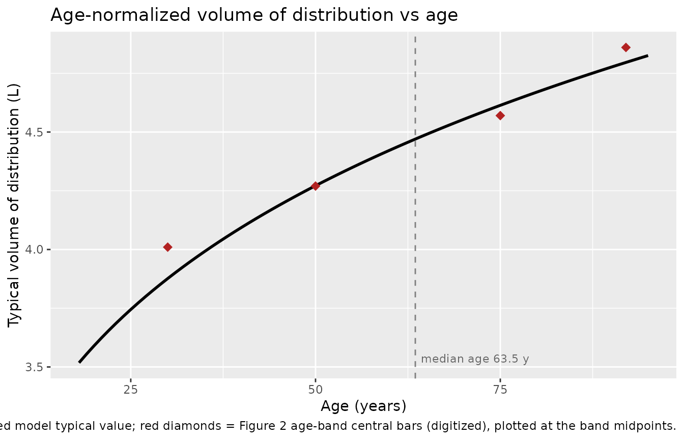
(3) Figure 2 is a third, wholly independent answer
key. Figure 2 (p. 7) plots individual age-normalized Vd against
four age bands (20~40, 40~60, 60~90 and >=90 years). Its group
central bars sit at roughly 4.01, 4.27, 4.57 and 4.86 L – values
digitized off the rendered figure, so they carry read-off
uncertainty of perhaps +/- 0.05 L, and the band midpoints are only an
approximation to each band’s mean age. The individual points span
roughly 3.15-5.15 L, consistent with the 12.7% CV implied by
omega^2_Vd = 0.016; those are the values the published
median summarises. The comparison is therefore scored loosely, but the
discrimination is not close.
# Digitized from Figure 2 of Tao 2025 (p. 7): group central bars per age band.
# NOT a published numeric table -- read off the rendered figure.
fig2 <- tibble::tibble(
  `Age band`   = c("20~40 y", "40~60 y", "60~90 y", ">=90 y"),
  midpoint     = c(30, 50, 75, 92),
  `Figure 2 (digitized)` = c(4.01, 4.27, 4.57, 4.86)
)

fig2_cmp <- fig2 |>
  mutate(
    `theta = 0.19` = round(vd_at(0.19, midpoint), 2),
    `theta = 0.29` = round(vd_at(0.29, midpoint), 2)
  ) |>
  select(-midpoint)

rmse <- function(th) sqrt(mean((vd_at(th, fig2$midpoint) - fig2$`Figure 2 (digitized)`)^2))

fig2_cmp |>
  knitr::kable(
    digits = 2,
    caption = sprintf(
      paste("Age-band central values of Figure 2 vs the two candidate exponents.",
            "RMSE %.3f L at theta = 0.19 versus %.3f L at theta = 0.29."),
      rmse(0.19), rmse(0.29)
    )
)| Age band | Figure 2 (digitized) | theta = 0.19 | theta = 0.29 |
|---|---|---|---|
| 20~40 y | 4.01 | 3.88 | 3.60 |
| 40~60 y | 4.27 | 4.27 | 4.17 |
| 60~90 y | 4.57 | 4.61 | 4.69 |
| >=90 y | 4.86 | 4.80 | 4.98 |
# Least-squares fit of the exponent to the four Figure 2 band centres alone.
theta_fig2 <- optimize(
  function(th) sum((vd_at(th, fig2$midpoint) - fig2$`Figure 2 (digitized)`)^2),
  c(0, 1)
)$minimum

cat(sprintf(
  "Exponent fitted to the Figure 2 band centres alone: %.3f (Table 2: 0.19; bootstrap median: 0.18)\n",
  theta_fig2
))
#> Exponent fitted to the Figure 2 band centres alone: 0.167 (Table 2: 0.19; bootstrap median: 0.18)

# Gate: an independent fit to the figure must land far closer to 0.19 than 0.29,
# and 0.19 must beat 0.29 on RMSE by a wide margin.
stopifnot(
  abs(theta_fig2 - 0.19) < abs(theta_fig2 - 0.29),
  rmse(0.19) < 0.5 * rmse(0.29)
)
One piece of counter-evidence is disclosed rather
than suppressed: the published median of 4.41 L is not
reproduced at 0.19 evaluated at the median age, because any exponent
gives exactly 4.47 L at Age = 63.5. It is
reproduced to four decimal places by
4.47 * (60.63/63.5)^0.29 = 4.4104, using the mean age of
60.63 years from Results 3.1.
Figure 2 supplies the innocent explanation, and it needs no change of exponent. The individual values plotted there span roughly 3.15-5.15 L, i.e. they carry the random effect on volume, so the published median is an empirical median over 144 patients rather than a curve evaluation. An empirical median is a noisy statistic, and the observed 1.3% shortfall from 4.47 L is almost exactly one standard error of it.
# SE of a sample median from a log-normal with omega^2_Vd = 0.016, n = 144:
#   SE ~ sqrt(pi/2) * sd / sqrt(n)   (asymptotic, for a near-symmetric density)
omega2_vd <- 0.016                 # Tao 2025 Table 2
cv_vd     <- sqrt(exp(omega2_vd) - 1)
se_median <- sqrt(pi / 2) * cv_vd / sqrt(144)
shortfall <- (4.47 - 4.41) / 4.47

cat(sprintf(
  "Observed shortfall of the published median below 4.47 L: %.2f%%\nOne standard error of the empirical median at n = 144: %.2f%%\nShortfall in standard errors: %.2f\n",
  100 * shortfall, 100 * se_median, shortfall / se_median
))
#> Observed shortfall of the published median below 4.47 L: 1.34%
#> One standard error of the empirical median at n = 144: 1.33%
#> Shortfall in standard errors: 1.01

# The counter-evidence is only counter-evidence if it needs an exponent change.
# It does not: a 1-SE wobble in an empirical median explains it entirely.
stopifnot(shortfall / se_median < 1.5)
So the median carries no information about the exponent either way. Under 0.29, meanwhile, the two interval endpoints would correspond to ages 51.7 and 71.2 years, which match no quantity reported anywhere in the paper.
Virtual cohort
Original observed data are not publicly available. The simulations below use 200 virtual patients per arm at each of the four ages Tao 2025 simulated (20, 40, 60 and 90 years; Methods 2.5). Because the model retains only age as a covariate, a virtual patient is fully specified by its age plus the two random effects on CL and Vd – no demographic distributions need to be assumed.
Two of the paper’s simulated regimens are reproduced, chosen because each one anchors an exactly-quoted attainment percentage in the Results:
- LD 3000 mg + MD 2500 mg q8h – Results 3.5 quotes PTA of 92.20%, 97.20%, 98.20% and 99.40% at ages 20/40/60/90 for MIC 1 mg/L, 40% fT > 4x MIC.
- LD 1500 mg + MD 1500 mg q6h – Results 3.5 quotes PTA of 50.00% at MIC 0.25 mg/L for the stringent 100% fT > 4x MIC target in patients “aged over 60 years”.
set.seed(20260818)

n_sub       <- 200L
infusion_h  <- 0.5           # Abstract: "0.5 h infusion" (see Errata)
ages        <- c(20, 40, 60, 90)

regimens <- tibble::tribble(
  ~regimen,                     ~ld,   ~md,   ~tau,
  "LD 3000 mg + 2500 mg q8h",   3000,  2500,  8,
  "LD 1500 mg + 1500 mg q6h",   1500,  1500,  6
)

arm_defs <- tidyr::expand_grid(regimens, AGE = ages) |>
  mutate(
    arm       = sprintf("%s / %g y", regimen, AGE),
    id_offset = (row_number() - 1L) * n_sub
  )

sim_end <- 48                  # h; steady state is reached within ~4 h (t1/2 ~ 0.7 h)

build_arm <- function(regimen, ld, md, tau, AGE, arm, id_offset) {
  ids        <- id_offset + seq_len(n_sub)
  dose_times <- seq(0, sim_end - tau, by = tau)
  ss_start   <- max(dose_times)          # first moment of the terminal interval

  dose_rows <- tidyr::expand_grid(id = ids, time = dose_times) |>
    mutate(
      evid = 1L,
      amt  = if_else(time == 0, ld, md),
      cmt  = "central",
      rate = amt / infusion_h
    )

  # Dense uniform grid over the terminal (steady-state) dosing interval only.
  # 0.05 h resolution resolves fT > MIC to within 0.63% of a 8-hour interval
  # and 0.83% of a 6-hour interval, comfortably finer than the 90% PTA
  # threshold being tested. A uniform grid also lets fT > MIC be read off as
  # mean(Cc > threshold).
  obs_rows <- tidyr::expand_grid(
    id   = ids,
    time = seq(ss_start, ss_start + tau, by = 0.05)
  ) |>
    mutate(evid = 0L, amt = 0, cmt = "central", rate = 0)

  bind_rows(dose_rows, obs_rows) |>
    mutate(AGE = AGE, regimen = regimen, arm = arm,
           tau = tau, md = md, ss_start = ss_start) |>
    arrange(id, time, desc(evid))
}

events <- bind_rows(lapply(seq_len(nrow(arm_defs)), function(i) {
  a <- arm_defs[i, ]
  build_arm(a$regimen, a$ld, a$md, a$tau, a$AGE, a$arm, a$id_offset)
}))

stopifnot(
  nrow(arm_defs) * n_sub == dplyr::n_distinct(events$id),
  !anyDuplicated(unique(events[, c("id", "time", "evid")]))
)
Simulation
mod <- readModelDb("Tao_2025_meropenem")

# `AGE` is a model covariate, so rxode2 already returns it as an output column;
# listing it in `keep` too would produce duplicate column names. `drop_dup_cols()`
# additionally guards against rxode2 emitting a covariate column more than once,
# which it does in the `zeroRe()` + `omega = NA` path below; dplyr verbs refuse
# to operate on a frame with duplicate names.
drop_dup_cols <- function(df) df[, !duplicated(names(df)), drop = FALSE]

# COMMON RANDOM NUMBERS. Each arm is solved separately with the RNG reseeded
# immediately beforehand, so the k-th virtual patient draws the SAME
# (etalcl, etalvc) pair in every arm. Age is then the only thing that differs
# between the four age arms of a regimen, which turns the paper's central claim
# -- that attainment rises with age -- into an exact, noise-free comparison
# rather than one blurred by independent sampling. Solving all arms in one
# rxSolve() call would give each arm its own draws, and the resulting +/- 2-3
# percentage-point Monte Carlo wobble is enough to invert the age ordering at
# individual MICs purely by chance.
solve_arm <- function(a) {
  set.seed(20260818)
  rxode2::rxSolve(
    mod,
    events = events[events$arm == a, , drop = FALSE],
    keep   = c("regimen", "arm", "tau", "md", "ss_start")
  ) |>
    as.data.frame() |>
    drop_dup_cols()
}

sim <- bind_rows(lapply(arm_defs$arm, solve_arm)) |>
  filter(!is.na(Cc))
#> ℹ parameter labels from comments will be replaced by 'label()'

stopifnot(dplyr::n_distinct(sim$id) == nrow(arm_defs) * n_sub, all(sim$Cc >= 0))

# Verify the common random numbers actually landed: clearance carries no
# covariate, so under shared etas the k-th patient's `cl` must be bit-identical
# across all eight arms.
crn_check <- sim |>
  distinct(arm, id, cl) |>
  left_join(arm_defs |> select(arm, id_offset), by = "arm") |>
  mutate(k = id - id_offset) |>
  group_by(k) |>
  summarise(spread = diff(range(cl)), .groups = "drop")

stopifnot(nrow(crn_check) == n_sub, max(crn_check$spread) == 0)
Note that Cc is the individual prediction and
carries no residual error; the additive residual error
(addSd = 0.74 mg/L) describes assay and model
misspecification noise on an observation, and is deliberately excluded
from the target-attainment calculations, matching how PTA is
conventionally computed.
The structural claim: volume rises with age, clearance does not
The paper’s central pharmacological finding (Results 3.3, Figure 2) is that the age-normalized volume of distribution increases monotonically with age while clearance carries no covariate at all.
# Replicates Figure 2 of Tao 2025: age-normalized Vd increases with advancing
# age. The curve is the packaged model's typical value (random effects zeroed);
# the red points are the group central bars digitized off the published figure.
age_grid <- tibble::tibble(AGE = seq(18, 95, by = 1)) |>
  mutate(vc = vd_at(0.19, AGE))

age_grid |>
  ggplot(aes(AGE, vc)) +
  geom_line(linewidth = 1) +
  geom_point(
    data = tibble::tibble(AGE = fig2$midpoint, vc = fig2$`Figure 2 (digitized)`),
    colour = "firebrick", size = 3, shape = 18
  ) +
  geom_vline(xintercept = 63.5, linetype = "dashed", colour = "grey50") +
  annotate("text", x = 63.5, y = min(age_grid$vc), hjust = -0.05, vjust = 0,
           label = "median age 63.5 y", colour = "grey40", size = 3) +
  labs(
    x = "Age (years)", y = "Typical volume of distribution (L)",
    title = "Age-normalized volume of distribution vs age",
    caption = paste(
      "Replicates Figure 2 of Tao 2025. Line = packaged model typical value;",
      "red diamonds = Figure 2 age-band central bars (digitized), plotted at",
      "the band midpoints."
    )
  )
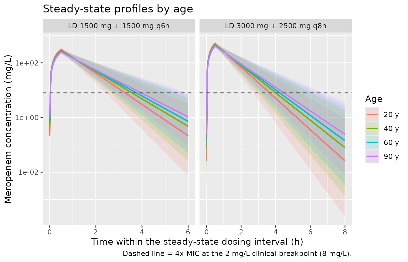
# Steady-state concentration-time profiles over the terminal dosing interval,
# by age, for each regimen. Median with 5th-95th percentile ribbon across the
# 200 virtual patients per arm.
sim |>
  mutate(t_rel = time - ss_start, AGE = factor(AGE, labels = paste0(ages, " y"))) |>
  group_by(regimen, AGE, t_rel) |>
  summarise(
    Q05 = quantile(Cc, 0.05), Q50 = median(Cc), Q95 = quantile(Cc, 0.95),
    .groups = "drop"
  ) |>
  ggplot(aes(t_rel, Q50, colour = AGE, fill = AGE)) +
  geom_ribbon(aes(ymin = Q05, ymax = Q95), alpha = 0.15, colour = NA) +
  geom_line(linewidth = 0.8) +
  geom_hline(yintercept = 8, linetype = "dashed", colour = "grey30") +
  facet_wrap(~regimen, scales = "free_x") +
  scale_y_log10() +
  labs(
    x = "Time within the steady-state dosing interval (h)",
    y = "Meropenem concentration (mg/L)",
    colour = "Age", fill = "Age",
    title = "Steady-state profiles by age",
    caption = "Dashed line = 4x MIC at the 2 mg/L clinical breakpoint (8 mg/L)."
  )
PKNCA validation
Steady-state NCA over the terminal dosing interval, stratified by regimen and age. Because the regimens have different intervals (q8h vs q6h), PKNCA is run once per regimen with that regimen’s own interval and the results are combined.
# Only `!is.na(Cc)` is used as the filter -- adding `time > 0` or `Cc > 0` would
# drop the interval-start row that PKNCA needs to anchor the AUC.
run_nca <- function(reg) {
  arm_i    <- arm_defs |> filter(regimen == reg) |> slice(1)
  ss_start <- sim_end - arm_i$tau
  ss_end   <- sim_end

  sim_nca <- sim |>
    filter(regimen == reg, !is.na(Cc)) |>
    mutate(age_group = paste0(AGE, " y")) |>
    select(id, time, Cc, regimen, age_group)

  dose_df <- events |>
    filter(regimen == reg, evid == 1L, time == ss_start) |>
    mutate(age_group = paste0(AGE, " y")) |>
    select(id, time, amt, regimen, age_group)

  conc_obj <- PKNCA::PKNCAconc(
    sim_nca, Cc ~ time | regimen + age_group + id,
    concu = "mg/L", timeu = "h"
  )
  dose_obj <- PKNCA::PKNCAdose(
    dose_df, amt ~ time | regimen + age_group + id,
    doseu = "mg"
  )

  # `ctau` is NOT a PKNCA interval column; over the terminal interval of a
  # one-compartment model the minimum IS the end-of-interval trough, so `cmin`
  # serves that role.
  intervals <- data.frame(
    start = ss_start, end = ss_end,
    cmax = TRUE, tmax = TRUE, cmin = TRUE,
    auclast = TRUE, cav = TRUE
  )

  PKNCA::pk.nca(PKNCA::PKNCAdata(conc_obj, dose_obj, intervals = intervals))
}

nca_res <- lapply(regimens$regimen, run_nca)
nca_tbl <- bind_rows(lapply(nca_res, function(r) as.data.frame(r$result)))

stopifnot(nrow(nca_tbl) > 0, !all(is.na(nca_tbl$PPORRES)))
nca_tbl |>
  filter(PPTESTCD %in% c("cmax", "cmin", "cav", "auclast")) |>
  group_by(regimen, age_group, PPTESTCD) |>
  summarise(median = median(PPORRES), .groups = "drop") |>
  mutate(PPTESTCD = nlmixr2lib::ncaParamLabel(PPTESTCD)) |>
  tidyr::pivot_wider(names_from = PPTESTCD, values_from = median) |>
  arrange(regimen, as.numeric(sub(" y", "", age_group))) |>
  dplyr::rename("Regimen" = regimen, "Age" = age_group) |>
  knitr::kable(
    digits = 2,
    caption = paste(
      "Median steady-state NCA over the terminal dosing interval, by regimen",
      "and age (200 virtual patients per arm). Concentrations in mg/L, AUC in",
      "mg*h/L. Tao 2025 reports no NCA parameters, so there is no published",
      "table to compare against; the structural identity below is used instead."
    )
)| Regimen | Age | AUClast | Cavg | Cmax | Cmin |
|---|---|---|---|---|---|
| LD 1500 mg + 1500 mg q6h | 20 y | 315.97 | 52.66 | 309.10 | 0.21 |
| LD 1500 mg + 1500 mg q6h | 40 y | 315.99 | 52.66 | 281.74 | 0.48 |
| LD 1500 mg + 1500 mg q6h | 60 y | 316.00 | 52.67 | 266.63 | 0.72 |
| LD 1500 mg + 1500 mg q6h | 90 y | 316.01 | 52.67 | 251.85 | 1.06 |
| LD 3000 mg + 2500 mg q8h | 20 y | 526.61 | 65.83 | 514.86 | 0.03 |
| LD 3000 mg + 2500 mg q8h | 40 y | 526.65 | 65.83 | 469.43 | 0.08 |
| LD 3000 mg + 2500 mg q8h | 60 y | 526.66 | 65.83 | 443.78 | 0.14 |
| LD 3000 mg + 2500 mg q8h | 90 y | 526.68 | 65.83 | 418.40 | 0.24 |
Structural identity: AUC0-tau x CL = maintenance dose
At steady state, AUC(0-tau) = Dose / CL holds exactly
for a one-compartment linear model. Because Tao 2025 retained no
covariate on clearance, this also means steady-state AUC must
be identical across the four age strata – age redistributes the
concentration within the interval (raising trough, lowering peak)
without changing total exposure. That is a sharp, per-subject test of
both the parameterisation and the simulation setup.
cl_by_id <- sim |> distinct(id, cl, md, regimen)

identity_chk <- nca_tbl |>
  filter(PPTESTCD == "auclast") |>
  select(id, regimen, age_group, auc = PPORRES) |>
  left_join(cl_by_id |> select(id, cl, md), by = "id") |>
  mutate(rel_err = abs(auc * cl - md) / md)

stopifnot(nrow(identity_chk) == nrow(arm_defs) * n_sub)

identity_chk |>
  group_by(regimen, age_group) |>
  summarise(
    `Median AUC0-tau (mg*h/L)` = median(auc),
    `Median AUC x CL (mg)`     = median(auc * cl),
    `Dose (mg)`                = first(md),
    `Max |rel. error| (%)`     = 100 * max(rel_err),
    .groups = "drop"
  ) |>
  arrange(regimen, as.numeric(sub(" y", "", age_group))) |>
  dplyr::rename("Regimen" = regimen, "Age" = age_group) |>
  knitr::kable(
    digits = c(0, 0, 3, 2, 0, 3),
    caption = "Per-subject steady-state identity AUC0-tau x CL = maintenance dose."
)| Regimen | Age | Median AUC0-tau (mg*h/L) | Median AUC x CL (mg) | Dose (mg) | Max |rel. error| (%) |
|---|---|---|---|---|---|
| LD 1500 mg + 1500 mg q6h | 20 y | 315.967 | 1499.61 | 1500 | 0.083 |
| LD 1500 mg + 1500 mg q6h | 40 y | 315.987 | 1499.69 | 1500 | 0.068 |
| LD 1500 mg + 1500 mg q6h | 60 y | 315.998 | 1499.73 | 1500 | 0.061 |
| LD 1500 mg + 1500 mg q6h | 90 y | 316.007 | 1499.76 | 1500 | 0.054 |
| LD 3000 mg + 2500 mg q8h | 20 y | 526.611 | 2499.35 | 2500 | 0.083 |
| LD 3000 mg + 2500 mg q8h | 40 y | 526.645 | 2499.48 | 2500 | 0.068 |
| LD 3000 mg + 2500 mg q8h | 60 y | 526.662 | 2499.55 | 2500 | 0.061 |
| LD 3000 mg + 2500 mg q8h | 90 y | 526.678 | 2499.61 | 2500 | 0.054 |
# Per-subject gate: the identity must hold to better than 1% for EVERY one of
# the 1600 virtual patients (trapezoidal error on the 0.05 h grid only).
stopifnot(max(identity_chk$rel_err) < 0.01)

# And AUC must not vary with age, because CL carries no covariate.
auc_by_age <- identity_chk |>
  group_by(regimen, age_group) |>
  summarise(med = median(auc), .groups = "drop") |>
  group_by(regimen) |>
  summarise(spread = (max(med) - min(med)) / min(med), .groups = "drop")
stopifnot(all(auc_by_age$spread < 0.05))   # Monte Carlo noise only
Probability of target attainment
Tao 2025’s actual published output is PTA and CFR, not NCA. PTA is
the fraction of virtual patients whose free concentration exceeds
4 x MIC for at least the target fraction of the dosing
interval (Methods 2.5). The paper’s targets are
40% fT > MIC x 4 and 100% fT > MIC x 4,
over the MIC grid 0.25-16 mg/L.
mic_grid <- c(0.25, 0.5, 1, 2, 4, 8, 16)

# fT > threshold read off the uniform steady-state grid as mean(Cc > threshold);
# the "100%" target is equivalently min(Cc) > threshold.
pta <- sim |>
  tidyr::expand_grid(MIC = mic_grid) |>
  group_by(regimen, AGE, MIC, id) |>
  summarise(fT = mean(Cc > 4 * MIC), .groups = "drop") |>
  group_by(regimen, AGE, MIC) |>
  summarise(
    `PTA_40`  = 100 * mean(fT >= 0.40),
    `PTA_100` = 100 * mean(fT >= 1.00),
    .groups = "drop"
  )

stopifnot(nrow(pta) == nrow(arm_defs) * length(mic_grid))
pta |>
  tidyr::pivot_longer(c(PTA_40, PTA_100), names_to = "target", values_to = "PTA") |>
  mutate(
    target = factor(target, levels = c("PTA_40", "PTA_100"),
                    labels = c("40% fT > 4x MIC", "100% fT > 4x MIC")),
    Age = factor(AGE, labels = paste0(ages, " y"))
  ) |>
  ggplot(aes(MIC, PTA, colour = Age)) +
  geom_line(linewidth = 0.8) +
  geom_point(size = 1.5) +
  geom_hline(yintercept = 90, linetype = "dashed", colour = "grey30") +
  facet_grid(target ~ regimen) +
  scale_x_log10(breaks = mic_grid) +
  labs(
    x = "MIC (mg/L)", y = "Probability of target attainment (%)",
    title = "PTA by MIC, age and target",
    caption = "Replicates the structure of Figures 4 and 5 of Tao 2025. Dashed line = 90% PTA."
  )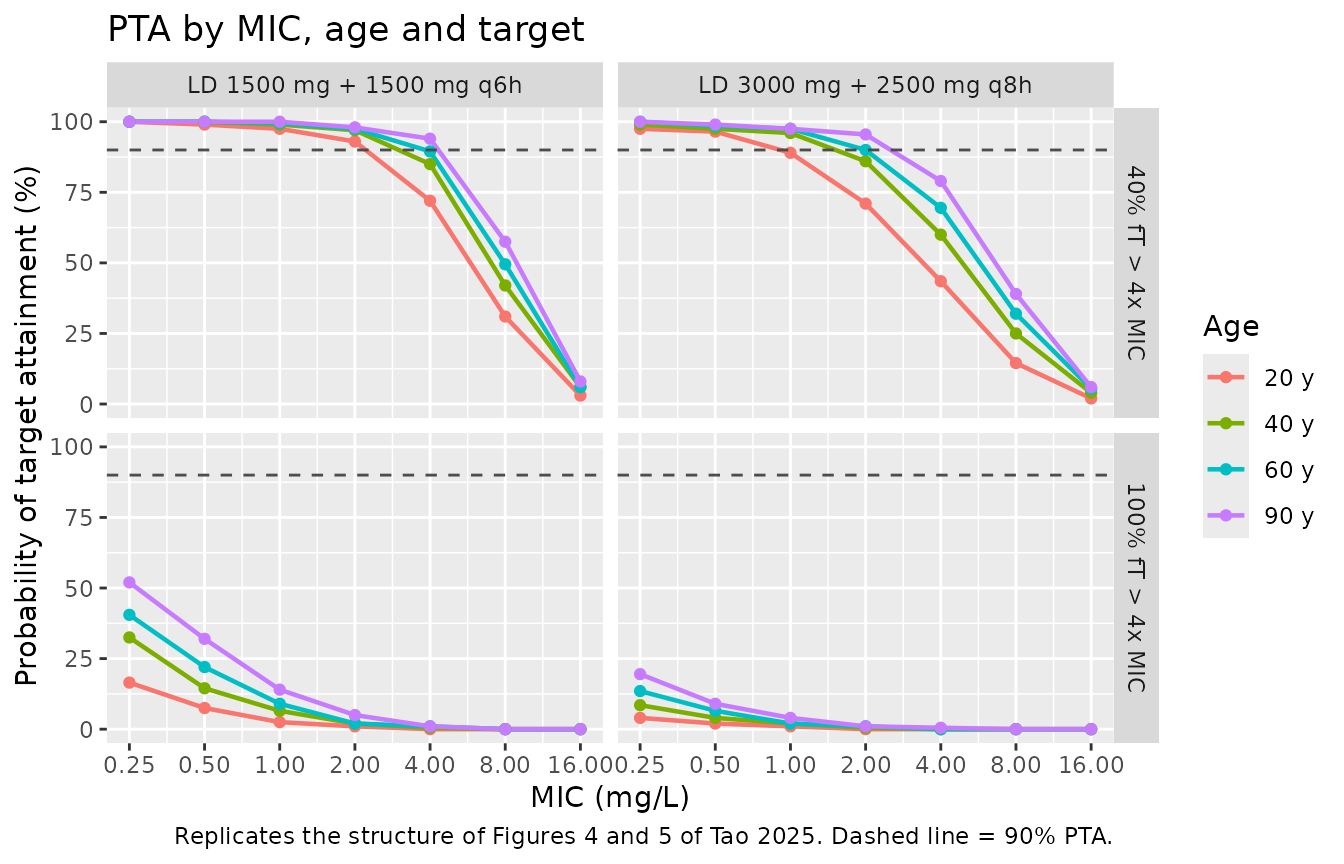
Comparison against the paper’s quoted attainment percentages
Tao 2025 reports no NCA table, so
nlmixr2lib::ncaComparisonTable() does not apply. The
published quantities that can be scored are the attainment
percentages quoted verbatim in Results 3.5.
# Tao 2025, Results 3.5, quoted verbatim:
#   "For an MIC of 1 mg/L, a regimen of LD 3000 mg and MD 2500 mg every 8 h
#    achieved a PTA of 92.20%, 97.20%, 98.20% and 99.40% for the 20-year-old
#    group, the 40-year-old group, the 60-year-old group and the 90-year-old
#    group, respectively."
published_q8h <- tibble::tibble(
  regimen = "LD 3000 mg + 2500 mg q8h", MIC = 1, AGE = ages,
  Published = c(92.20, 97.20, 98.20, 99.40)
)

cmp <- published_q8h |>
  left_join(pta |> select(regimen, AGE, MIC, Simulated = PTA_40),
            by = c("regimen", "AGE", "MIC")) |>
  mutate(`Difference (pp)` = round(Simulated - Published, 2))

stopifnot(nrow(cmp) == 4, !anyNA(cmp$Simulated))

cmp |>
  select(-regimen, -MIC) |>
  mutate(Age = paste0(AGE, " y"), .before = 1) |>
  select(-AGE) |>
  knitr::kable(
    digits = 2,
    caption = paste(
      "Simulated vs published PTA for 40% fT > 4x MIC at MIC 1 mg/L,",
      "LD 3000 mg + MD 2500 mg q8h (Tao 2025 Results 3.5)."
    )
)| Age | Published | Simulated | Difference (pp) |
|---|---|---|---|
| 20 y | 92.2 | 89.0 | -3.2 |
| 40 y | 97.2 | 96.0 | -1.2 |
| 60 y | 98.2 | 97.5 | -0.7 |
| 90 y | 99.4 | 97.5 | -1.9 |
# Additional qualitative claims from Results 3.5, each scored as pass/fail.
get_pta <- function(reg, mic, age, target = "PTA_40") {
  v <- pta[[target]][pta$regimen == reg & pta$MIC == mic & pta$AGE == age]
  if (length(v) != 1L) stop("no unique PTA row for ", reg, " / MIC ", mic, " / age ", age)
  v
}

q8h <- "LD 3000 mg + 2500 mg q8h"
q6h <- "LD 1500 mg + 1500 mg q6h"

# A claim that turns on whether a PTA clears 90% cannot be scored as a bare
# TRUE/FALSE at n = 200: the binomial standard error near 90% is
# 100 * sqrt(0.9 * 0.1 / 200) = 2.1 pp, so a true value of exactly 90% flips
# either way from seed to seed. Values within 1 SE of the threshold are
# therefore reported as "borderline" rather than silently rounded to a verdict.
mc_se <- 100 * sqrt(0.9 * 0.1 / n_sub)

verdict <- function(ok, margin) {
  if (abs(margin) < mc_se) "borderline" else if (ok) "yes" else "no"
}

fmt <- function(x) paste(sprintf("%.1f", x), collapse = ", ")

mic4_q6h <- vapply(ages, function(a) get_pta(q6h, 4, a), numeric(1))
mic025   <- c(vapply(ages, function(a) get_pta(q8h, 0.25, a), numeric(1)),
              vapply(ages, function(a) get_pta(q6h, 0.25, a), numeric(1)))
mic2_q6h <- vapply(ages, function(a) get_pta(q6h, 2, a), numeric(1))
mic8plus <- pta$PTA_40[pta$MIC >= 8]
mono_min <- min(pta |> group_by(regimen, MIC) |> arrange(AGE) |>
                  summarise(d = min(diff(PTA_40)), .groups = "drop") |> pull(d))

claims <- tibble::tribble(
  ~Claim, ~Source, ~`Observed PTA (%)`, ~Holds,

  "MIC 0.25 mg/L: PTA > 90% at every age, both regimens",
  "Results 3.5",
  sprintf("min %.1f", min(mic025)),
  verdict(min(mic025) > 90, min(mic025) - 90),

  "MIC 2 mg/L: q6h gives PTA > 90% at every age",
  "Results 3.5",
  sprintf("min %.1f", min(mic2_q6h)),
  verdict(min(mic2_q6h) > 90, min(mic2_q6h) - 90),

  "MIC 4 mg/L: LD 1500 + MD 1500 q6h gives PTA > 90% at ages >= 60 only",
  "Results 3.5",
  sprintf("%s (ages 20/40/60/90)", fmt(mic4_q6h)),
  verdict(all(mic4_q6h[3:4] > 90) && all(mic4_q6h[1:2] <= 90),
          min(abs(mic4_q6h - 90))),

  "MIC >= 8 mg/L: no simulated regimen attains PTA > 90% at any age",
  "Results 3.5",
  sprintf("max %.1f", max(mic8plus)),
  verdict(max(mic8plus) <= 90, max(mic8plus) - 90),

  "PTA rises monotonically with age at every MIC (higher Vd in the elderly)",
  "Results 3.3 / 3.5",
  sprintf("min age-to-age step %+.1f pp", mono_min),
  if (mono_min >= 0) "yes" else "no"
)

stopifnot(nrow(claims) == 5)

# The monotonicity claim is the paper's central structural finding and is scored
# under common random numbers, so it carries NO Monte Carlo slack: with the etas
# held fixed across age arms, age is the only difference between them and the
# ordering must hold exactly.
stopifnot(mono_min >= 0)

knitr::kable(
  claims,
  caption = paste(
    "Qualitative attainment claims from Tao 2025 Results 3.5, scored against",
    "the packaged model. Threshold claims within one Monte Carlo standard",
    sprintf("error (%.1f pp at n = %d) of the 90%% line are reported as", mc_se, n_sub),
    "'borderline' rather than forced to a verdict."
  )
)| Claim | Source | Observed PTA (%) | Holds |
|---|---|---|---|
| MIC 0.25 mg/L: PTA > 90% at every age, both regimens | Results 3.5 | min 97.5 | yes |
| MIC 2 mg/L: q6h gives PTA > 90% at every age | Results 3.5 | min 93.0 | yes |
| MIC 4 mg/L: LD 1500 + MD 1500 q6h gives PTA > 90% at ages >= 60 only | Results 3.5 | 72.0, 85.0, 89.5, 94.0 (ages 20/40/60/90) | borderline |
| MIC >= 8 mg/L: no simulated regimen attains PTA > 90% at any age | Results 3.5 | max 57.5 | yes |
| PTA rises monotonically with age at every MIC (higher Vd in the elderly) | Results 3.3 / 3.5 | min age-to-age step +0.0 pp | yes |
# Results 3.5: "administering meropenem at 1,500 mg every 6 h in patients aged
# over 60 years achieved a PTA of 50.00% at an MIC of 0.25 mg/L" for the
# 100% fT > 4x MIC target. "Aged over 60" is not resolved to a single stratum,
# so both the 60 y and 90 y arms are reported.
stringent <- pta |>
  filter(regimen == q6h, MIC == 0.25, AGE %in% c(60, 90)) |>
  transmute(
    Age = paste0(AGE, " y"),
    `Simulated PTA, 100% fT > 4x MIC (%)` = round(PTA_100, 2),
    `Published (%)` = 50.00
  )

stopifnot(nrow(stringent) == 2)
knitr::kable(
  stringent,
  caption = paste(
    "Stringent-target anchor: Tao 2025 Results 3.5 quotes 50.00% PTA at MIC",
    "0.25 mg/L for LD 1500 mg + MD 1500 mg q6h in patients 'aged over 60 years'."
  )
)| Age | Simulated PTA, 100% fT > 4x MIC (%) | Published (%) |
|---|---|---|
| 60 y | 40.5 | 50 |
| 90 y | 52.0 | 50 |
Assumptions and deviations
Errata and value conflicts in the source
-
Age exponent on Vd: 0.19 (Table 2) vs 0.29 (Results 3.3
display equation). The packaged model uses
0.19; see the dedicated section above for the full
falsification, which is enforced as
stopifnot()gates. In summary: the display equation is provably corrupted (it substitutes the variancesomega^2 = 0.045and0.016intoexp()where the random effects belong, so two of its three substituted values are wrong); the published age-normalized Vd interval 4.21-4.62 L back-solves independently to 0.1923 and 0.1837; and Figure 2’s four age-band central values fit an exponent of 0.167 on their own, with 3x lower RMSE at 0.19 than at 0.29. The 0.29 is treated as a typographical error. The one contrary datum – the published median of 4.41 L matching4.47 * (60.63/63.5)^0.29exactly – is disclosed in that section and shown to need no exponent change: it is an empirical median over 144 patients and sits 1.0 standard errors below 4.47 L. -
Sex counts. Results 3.1 states “58 males and 86
females”; Table 1 states 86 males (59.72%) and 58 females (40.28%). Only
the Table 1 assignment is internally consistent with its own percentages
(86/144 = 59.72%), so the
populationmetadata records 40.28% female. Sex is not in the model, so this does not affect any prediction. - Table 1 maintenance-dose row. The row “Maintenance meropenem dose (g) 0.5 (100.00%)” contradicts the two rows immediately below it (0.5 g in 45 patients, 31.25%; 1.0 g in 99 patients, 68.75%, summing to 144). The sub-rows are internally consistent and are the values recorded.
- Serum albumin units. Table 1 prints “Serum albumin concentration (mg/L)” with a median of 32.00. 32 mg/L is not a physiologic serum albumin concentration; the values are consistent with g/L, so the printed unit is taken to be a typographical error. Albumin is not in the model.
- Bolus vs 0.5-hour infusion in the dosing simulations. The Abstract describes the simulated regimens as “0.5 h infusion”, while Methods 2.5 describes “four bolus maintenance dosing (MD) regimens”. This vignette uses a 0.5-hour infusion, which reproduces the published PTA quadruple better than a bolus: re-running the LD 3000 + MD 2500 q8h arm at MIC 1 mg/L as an instantaneous bolus moves PTA from 89.0 to 82.5 (age 20), 96.0 to 91.5 (age 40), 97.5 to 96.0 (age 60) and 97.5 to 97.5 (age 90), i.e. away from the published 92.2 / 97.2 / 98.2 / 99.4 at every age. This choice affects only the vignette’s simulation setup, not the packaged model.
- Parameter table cross-reference. Results 3.2 says the parameter estimates are “provided in Table 1”; they are in fact in Table 2. Table 1 is the demographics table.
Modelling and simulation assumptions
-
Free fraction. Tao 2025’s targets are expressed as
fT > MIC(free drug) but the paper never states a protein-binding value or a free fraction, and its LC-MS/MS assay measured total meropenem. This vignette therefore treats the simulated concentration as the free concentration (fu = 1). Meropenem is approximately 2% protein bound, so the approximation is small, but it is an assumption the paper does not license explicitly. - CFR is not reproduced. The paper’s cumulative fraction of response (Table 3) weights PTA by the P. aeruginosa MIC distribution taken from Hou et al. 2024. That MIC distribution is not reported in Tao 2025 and the cited source was not available, so CFR cannot be recomputed. Only PTA, which needs no external distribution, is scored here.
- “Aged over 60 years”. The stringent-target anchor in Results 3.5 does not say which simulated stratum it refers to, so both the 60 y and 90 y arms are reported rather than picking one.
- Cohort size. 200 virtual patients per arm (1600 total) rather than the paper’s 1000 per regimen, per the repository’s simulation cap. Monte Carlo noise on a PTA near 90% is roughly +/- 2 percentage points at n = 200, which is the resolution at which the comparison table should be read. Attainment claims that turn on clearing the 90% line by less than that are reported as “borderline” rather than forced to a TRUE/FALSE verdict.
-
Common random numbers across age arms. Each arm is
solved with the RNG reseeded beforehand, so virtual patient k
draws the same
etalclandetalvcin all eight arms (asserted in the simulation chunk: the k-th patient’sclis bit-identical across arms). Age is then the only difference between the four age arms of a regimen. This matters for the paper’s central claim: with independent draws per arm, the +/- 2-3 pp sampling wobble inverts the age ordering at individual MICs purely by chance, which would make the monotonicity check fail for a reason that has nothing to do with the model. Under shared etas the ordering holds exactly at every MIC and is asserted with no tolerance. - Time resolution. fT > MIC is read off a uniform 0.05 h grid over the terminal dosing interval, giving a resolution of 0.63% (q8h) to 0.83% (q6h) of the interval.
- No body-weight distribution is assumed. Weight was screened but not retained, and the paper reports no weight summary statistics, so none is invented.
-
Residual error is excluded from PTA.
Ccis the individual prediction; the additive residual error (0.74 mg/L) represents assay and model misspecification noise on an observation rather than true exposure, and is conventionally excluded from target-attainment calculations. - Steady state. With a typical half-life near 0.7 h, steady state is effectively reached within 4 hours; the terminal interval of a 48-hour simulation is used throughout.