Venetoclax + azacitidine in myelodysplastic syndromes (Thakre 2025)
Source:vignettes/articles/Thakre_2025_venetoclax.Rmd
Thakre_2025_venetoclax.RmdModel and source
- Citation: Thakre N, Maier C, Zha J, Engelhardt B, Wolff JE, Mensing S. Semi-mechanistic population PK/PD model to aid clinical understanding of myelodysplastic syndromes following treatment with Venetoclax and Azacitidine. CPT Pharmacometrics Syst Pharmacol. 2025;14(3):448-458. doi:10.1002/psp4.13284. PD parameter values from Table 2; PK parameter values from Supplementary Table S1; model structure from the NONMEM control stream in the Supporting Information (Data S1). The legacy PK model is Jones AK et al., AAPS J 2016;18(5):1192-1202, doi:10.1208/s12248-016-9927-9.
- Description: Semi-mechanistic population PK/PD model of venetoclax plus azacitidine in treatment-naive adults with higher-risk myelodysplastic syndromes (MDS). PK: two-compartment venetoclax model with first-order absorption, an absorption lag and first-order elimination (the legacy venetoclax model re-estimated in MDS), with food and a power function of dose on relative bioavailability, CYP3A / OATP1B3 inhibitors and rituximab on CL/F, and sex and patient status on V2/F. PD: normal and MDS hematopoietic stem cells in the bone marrow differentiate into three parallel Friberg-type lineages (neutrophils, platelets, red blood cells; proliferating precursor, three transit compartments, circulating pool) with feedback from the circulating counts relative to healthy reference values. MDS stem cells proliferate faster and differentiate 100-fold less than normal stem cells; marrow crowding raises apoptosis of every marrow cell type. Venetoclax concentration linearly increases apoptosis of normal and MDS stem cells and of neutrophil and platelet precursors; azacitidine (an on/off flag, days 1-7 of each 28-day cycle) lowers proliferation of stem cells and of neutrophil and platelet precursors. Outputs: venetoclax Cc, percent bone-marrow blasts, and blood neutrophil, platelet and red blood cell counts.
- Article: https://doi.org/10.1002/psp4.13284 (open access; PMC11919261)
Thakre et al. built a joint semi-mechanistic PK/PD model of venetoclax given with azacitidine to patients with previously untreated higher-risk myelodysplastic syndromes (MDS). The venetoclax PK model is the legacy two-compartment model (Jones 2016) re-estimated in MDS with the legacy estimates as an informative prior (Supplementary Table S1). The PD model is a Friberg-type hematopoiesis model extended to three parallel lineages (neutrophils, platelets, red blood cells) fed by normal and MDS stem cells in the bone marrow, with bone-marrow crowding and feedback relative to healthy reference counts (Figure 1; full NONMEM code in Data S1). The model was fitted simultaneously to bone-marrow blast percentages and to blood neutrophil, platelet and red blood cell counts over the first five 28-day cycles.
Population
The model was developed from 57 patients with treatment-naive higher-risk MDS in the phase 1b study NCT02942290 (data cut-off 21 August 2019; Table 1): median age 71 years (range 26-85), 75% male, 96% White, median body weight 82.5 kg. Baseline bone-marrow blasts were 1-23% (median 12%); baseline neutrophils 0.11-6.58 x 10^9/L (median 0.86), platelets 5-430 x 10^9/L (median 57) and red blood cells 1.58-4.30 x 10^12/L (median 2.98). Ten patients received venetoclax 400 or 800 mg daily for 28 of 28 days (original protocol), two received azacitidine alone, and the rest received venetoclax 100, 200 or 400 mg daily for 14 of 28 days (revised protocol); azacitidine 75 mg/m^2 was given on days 1-7 of every cycle. The data comprised 342 venetoclax concentrations, 242 bone-marrow blast samples and 1940 / 1951 / 1780 neutrophil / platelet / red blood cell counts.
The same information is available programmatically via
readModelDb("Thakre_2025_venetoclax")()$population.
Source trace
Every ini() value carries an in-file comment pointing to
its source. The table below collects them. “S1 code” is the NONMEM
control stream printed in the Supporting Information (Data S1).
| Equation / parameter | Value | Source location |
|---|---|---|
ka, CL/F, V2/F,
Q/F, V3/F
|
3.71 1/day, 451 L/day, 117 L, 98.0 L/day, 120 L | Table S1 |
absorption lag tlag
|
0.0533 day | Table S1 ‘Lag time in absorption’ |
| food effects on F1 (fasting / moderate / high / any meal vs low fat) | 0.334 / 1.32 / 1.43 / 1.22 | Table S1 |
dose nonlinearity on F1, (DOSE/400)^e
|
-0.183 | Table S1; S1 code F1 = F1ETA*(DOSE/400)**(-0.183)
|
| moderate / strong CYP3A inhibitor on CL/F | 0.819 / 0.175 | Table S1 |
| OATP1B3 inhibitor on CL/F | 0.853 | S1 code only (IF(OATP_HIB.GE.1) CL = CL*0.853) |
| rituximab on CL/F | 1.22 | Table S1 |
| female sex / patient (vs healthy) on V2/F | 0.689 / 1.70 | Table S1; S1 code IF(SEX.EQ.1) V2 = V2*0.689
|
| IIV CL/F, V2/F, F1 (variance) | 0.160, 0.203, 0.0935 | Table S1 |
| PK residual error (variance) | proportional 0.222, additive 3.07e-7 | Table S1 |
| MTTP, kdel,P, kdel,P1 | 57.7 h, 0.0220 1/day, 32.7 1/day | Table 2 |
| MTTN, kdel,N, kdel,N1 | 287 h, 0.536 1/day, 0.690 1/day | Table 2 |
| MTTR, kdel,R, kdel,R1 | 36.7 h, 0.00183 1/day, 0.460 1/day | Table 2 |
| kprol,S | 0.781 1/day | Table 2 |
| kmat,P / kmat,N / kmat,R | 2.02e-5 / 0.00292 / 0.00776 1/day | Table 2 |
| fp (increased MDS proliferation) | 0.000113 | Table 2; Methods kprol,MDS = (1 + fp) kprol,S
|
| venetoclax slopes SLPS / SLPMDS / SLPN1 / SLPP1 | 0.169 / 0.140 / 0.241 / 0.543 L/mg | Table 2 |
| azacitidine multiplier on stem cells, alphaSMDS | 0.760 | Table 2; S1 code DEAZA = 1/(1+10**(MU_15+ETA(15)))
|
| azacitidine multiplier on N / P precursors, alphaN1P1 | 0.788 | Table 2; S1 code
DEAZAB = 1-1/(2+10**(MU_19+ETA(19)))
|
| PD IIV | Table 2 %CV, converted below | Table 2 (footnote formula) |
| PD residual error (variance) | blasts 0.859, neutrophils 0.0914, platelets 0.0424, RBC 0.00202 | Table 2 |
| feedback exponents gamma / gammaN | 0.125 / 0.148 | Methods; S1 code GAM, GAMN
|
| fdiff (impaired MDS differentiation) | 0.01 | S1 code IMPDIFF = 0.01
|
| initial normal stem cells / MDS stem cells | 0.1 | S1 code FNORM = 0.1
|
| marrow mononuclear cells | 10^12 | S1 code A05 = (PERBLA/100)*1E12/1E9
|
| blood volume | 5 L | S1 code VPB = 5
|
| healthy reference counts HBP / HBN / HBR | 300 / 5.15 / 5400 x 10^9/L | S1 code HBP, HBN, HBR
|
d/dt(depot), d/dt(central),
d/dt(peripheral1)
|
n/a | S1 code $DES DADT(1)-DADT(3) |
d/dt(hsc), d/dt(hsc_mds)
|
n/a | S1 code DADT(4), DADT(5); Methods kprol,MDS,
kmat,MDS, fcrowd
|
| neutrophil / platelet / RBC chains | n/a | S1 code DADT(7)-DADT(21) |
steady-state initial conditions, kprol_*,
kdel_stem, kdel_mds
|
n/a | S1 code KPROLP, KPROLN,
KPROLR, A07, A012,
A017, DEL, DELMDS
|
| crowding and feedback | n/a | Methods equations; S1 code CROWD, FBNE,
FBPL, FBRE
|
| observation transforms | n/a | S1 code $ERROR (logit of percent blasts; log10
counts) |
PD parameterisation. The source writes every PD
parameter as 10^(THETA + ETA). Table 2 prints the typical
values on the natural scale; the model stores them as natural
logarithms. Table 2 gives IIV as a %CV, with the footnote formula %CV =
sqrt(exp(omega^2) - 1) x 100 applied to the base-10 ETA. Inverting that
gives omega^2 on the log10 scale, log(1 + CV^2), and the
model’s natural-log variance is that value times log(10)^2.
The log10-scale variances recovered this way are of the same size as the
diagonal of the $OMEGA block printed in Data S1, which
supports this reading.
The two azacitidine effects are the multipliers themselves, not the
THETAs. The Table 2 confidence interval of alphaN1P1, (0.715, 0.855), is
symmetric around 0.788 only on the THETA19 scale of
1 - 1/(2 + 10^THETA19). The printed lower bound of
alphaSMDS (0.698) is what 1/(1 + 10^THETA15) gives for
0.760 with a 15.9% RSE. The model therefore stores
log(1/0.760 - 1) and
log(1/(1 - 0.788) - 2).
Model structure
mod <- readModelDb("Thakre_2025_venetoclax")
mod_typical <- rxode2::zeroRe(mod)
#> ℹ parameter labels from comments will be replaced by 'label()'
Time is in days, venetoclax doses in mg and concentrations in mg/L. The PD states are cell numbers in units of 10^9 cells: blood counts are the circulating pools divided by a 5 L blood volume, and percent marrow blasts is the MDS stem-cell pool relative to 10^12 marrow mononuclear cells. Every lineage starts at the steady state implied by the patient’s own baseline counts; the source derives the precursor proliferation rates and the stem-cell apoptosis rates from that condition.
Azacitidine enters only as the time-varying flag
CONMED_AZACITIDINE, set to 1 on days 1-7 of every 28-day
cycle. The simulations below follow the source’s own simulation settings
(Methods): all patients male, venetoclax taken with a meal of unrecorded
type (“any meal”), no interacting co-medication.
cycle_len <- 28
n_cycles <- 5

# Event table for one subject. `ven_days` venetoclax doses per 28-day cycle
# (14 under the revised protocol, 28 under the original); `dose = 0` gives
# azacitidine monotherapy. Observation rows sit on the `central` ODE state with
# dvid = 1, which returns every endpoint column. The azacitidine flag changes
# at days 7 and 28 of each cycle, so those times are on the grid.
make_subject <- function(id, dose, ven_days = 14, grid_by = 1) {
  dose_times <- unlist(lapply(
    seq_len(n_cycles) - 1,
    function(k) k * cycle_len + seq_len(ven_days) - 1
  ))
  aza_switch <- unlist(lapply(seq_len(n_cycles) - 1, function(k) k * cycle_len + 7))
  obs_times <- sort(unique(c(seq(0, n_cycles * cycle_len, by = grid_by), aza_switch)))
  obs <- data.frame(id = id, time = obs_times, amt = 0, evid = 0L, cmt = "central", dvid = 1L)
  if (dose > 0) {
    doses <- data.frame(id = id, time = dose_times, amt = dose, evid = 1L, cmt = "depot", dvid = NA_integer_)
    obs <- dplyr::bind_rows(doses, obs)
  }
  obs |>
    dplyr::arrange(time, dplyr::desc(evid)) |>
    dplyr::mutate(
      CONMED_AZACITIDINE = as.integer((time %% cycle_len) < 7),
      # DOSE only scales F1 of venetoclax doses; any positive value is valid
      # for the azacitidine-only arm, which has no venetoclax dose records.
      DOSE = if (dose > 0) dose else 400
    )
}

# Covariates that are fixed across the simulations: male, 'any meal' with
# venetoclax, no CYP3A / OATP1B3 inhibitor, no rituximab, patients.
fixed_covs <- data.frame(
  SEXF = 0, FED = 1, FED_LOWFAT = 0, FED_MEDFAT = 0, FED_HIGHFAT = 0,
  CONMED_CYP3A4_INH_STRONG = 0, CONMED_CYP3A4_INH_MOD = 0,
  CONMED_OATP1B_INH = 0, CONMED_RITUX = 0, DIS_HEALTHY = 0
)

# Median baseline patient (Table 1).
median_patient <- data.frame(BMBLAST_PCT = 12, NEUT = 0.86, PLT_BASE = 57, RBC_BASE = 2.975)

arm_levels <- c("AZA monotherapy", "AZA + 100 mg Ven", "AZA + 200 mg Ven", "AZA + 400 mg Ven")
arm_dose <- c(0, 100, 200, 400)
Untreated steady state
Without venetoclax or azacitidine every lineage should stay at the
patient’s baseline. The only drift is the slow expansion of the MDS
clone (its apoptosis rate is set from the normal-stem-cell balance, so
it grows at fp x kprol,S per day, about 0.009% per day for
the typical patient).
ev_untreated <- make_subject(1, dose = 0) |>
  mutate(CONMED_AZACITIDINE = 0L) |>
  cbind(fixed_covs, median_patient)
ss <- rxode2::rxSolve(mod_typical, ev_untreated, returnType = "data.frame")
#> ℹ omega/sigma items treated as zero: 'etalcl', 'etalvc', 'etalfdepot', 'etalmtt_plt', 'etalkdel_plt', 'etalmtt_anc', 'etalkdel_anc', 'etalmtt_rbc', 'etalkdel_rbc', 'etalkprol_stem', 'etalkmat_plt', 'etalkmat_anc', 'etalkmat_rbc', 'etalfp_mds', 'etalslope_stem', 'etalslope_mds', 'etalslope_prol_anc', 'etalaza_stem', 'etalkdel_prol_plt', 'etalkdel_prol_anc', 'etalkdel_prol_rbc', 'etalaza_prol', 'etalslope_prol_plt'
ss_end <- ss |> filter(time == max(time))
ss_check <- tibble(
  endpoint = c("Blasts (%)", "Neutrophils (10^9/L)", "Platelets (10^9/L)", "RBC (10^12/L)"),
  baseline = c(12, 0.86, 57, 2.975),
  day_140 = c(ss_end$bmblast, ss_end$ANC, ss_end$PLT, ss_end$RBC)
) |>
  mutate(pct_change = 100 * (day_140 / baseline - 1))
knitr::kable(ss_check, digits = 3)| endpoint | baseline | day_140 | pct_change |
|---|---|---|---|
| Blasts (%) | 12.000 | 12.019 | 0.160 |
| Neutrophils (10^9/L) | 0.860 | 0.860 | -0.042 |
| Platelets (10^9/L) | 57.000 | 57.116 | 0.204 |
| RBC (10^12/L) | 2.975 | 2.974 | -0.035 |
# Deterministic typical-value solve against the baseline it was initialised
# at: a wrong steady-state formula (KPROL, A0x, DEL) moves the counts by tens
# of percent within days. The 1% bound admits the designed MDS expansion of
# ~1.2% over 140 days on the blast pool only.
stopifnot(
  all(abs(ss_check$pct_change[-1]) < 0.5),
  abs(ss_check$pct_change[1]) < 2
)
Typical-patient time courses
The median patient (Table 1 baselines) under the four regimens the source simulated (Figure 4): azacitidine alone on days 1-7, or with venetoclax 100, 200 or 400 mg once daily on days 1-14 of each 28-day cycle.
ev_typ <- bind_rows(lapply(seq_along(arm_dose), function(i) {
  make_subject(i, arm_dose[i], grid_by = 0.25) |> mutate(arm = arm_levels[i])
})) |>
  cbind(fixed_covs, median_patient)
sim_typ <- rxode2::rxSolve(mod_typical, ev_typ, keep = "arm", returnType = "data.frame", cores = 1L) |>
  mutate(arm = factor(arm, levels = arm_levels))
#> ℹ omega/sigma items treated as zero: 'etalcl', 'etalvc', 'etalfdepot', 'etalmtt_plt', 'etalkdel_plt', 'etalmtt_anc', 'etalkdel_anc', 'etalmtt_rbc', 'etalkdel_rbc', 'etalkprol_stem', 'etalkmat_plt', 'etalkmat_anc', 'etalkmat_rbc', 'etalfp_mds', 'etalslope_stem', 'etalslope_mds', 'etalslope_prol_anc', 'etalaza_stem', 'etalkdel_prol_plt', 'etalkdel_prol_anc', 'etalkdel_prol_rbc', 'etalaza_prol', 'etalslope_prol_plt'
#> Warning: multi-subject simulation without without 'omega'

sim_typ |>
  select(time, arm, `Blasts (%)` = bmblast, `Neutrophils (10^9/L)` = ANC,
         `Platelets (10^9/L)` = PLT, `RBC (10^12/L)` = RBC) |>
  pivot_longer(-c(time, arm)) |>
  ggplot(aes(time / cycle_len, value, colour = arm)) +
  geom_line() +
  facet_wrap(~name, scales = "free_y") +
  labs(x = "Cycle", y = NULL, colour = NULL,
       caption = "Typical-value predictions for the median patient of Table 1.") +
  theme(legend.position = "bottom")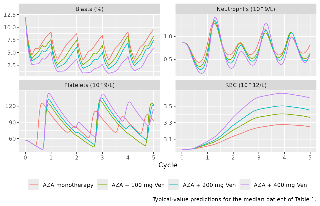
typ_end_c1 <- sim_typ |> filter(time == 28)
typ_blast <- setNames(typ_end_c1$bmblast, as.character(typ_end_c1$arm))
typ_end_c1 |> select(arm, bmblast, ANC, PLT, RBC) |> knitr::kable(digits = 3)| arm | bmblast | ANC | PLT | RBC |
|---|---|---|---|---|
| AZA monotherapy | 9.050 | 0.850 | 103.621 | 3.017 |
| AZA + 100 mg Ven | 7.595 | 0.704 | 119.445 | 3.038 |
| AZA + 200 mg Ven | 6.665 | 0.607 | 127.421 | 3.051 |
| AZA + 400 mg Ven | 5.150 | 0.462 | 139.274 | 3.074 |
# Deterministic: venetoclax adds apoptosis of MDS stem cells, so blasts at the
# end of cycle 1 fall with dose; at 400 mg the median patient reaches marrow
# remission (<= 5% and <= 50% of baseline).
stopifnot(
  typ_blast[["AZA + 400 mg Ven"]] < typ_blast[["AZA + 100 mg Ven"]],
  typ_blast[["AZA + 100 mg Ven"]] < typ_blast[["AZA monotherapy"]],
  typ_blast[["AZA + 400 mg Ven"]] <= 6
)
Venetoclax PK and PKNCA
Steady-state venetoclax exposure on cycle 1 day 14 (the 14th daily
dose) for the three venetoclax doses, typical values. The paper reports
no NCA, so the check is internal: at steady state the dosing-interval
AUC must equal F x Dose / CL.
pk_events <- bind_rows(lapply(2:4, function(i) {
  d <- arm_dose[i]
  doses <- data.frame(id = i, time = 0:13, amt = d, evid = 1L, cmt = "depot", dvid = NA_integer_)
  obs <- data.frame(id = i, time = c(0, seq(13, 14, by = 1 / 96)), amt = 0, evid = 0L,
                    cmt = "central", dvid = 1L)
  bind_rows(doses, obs) |>
    arrange(time, desc(evid)) |>
    mutate(treatment = paste(d, "mg"), DOSE = d, CONMED_AZACITIDINE = 0L)
})) |>
  cbind(fixed_covs, median_patient)
pk_sim <- rxode2::rxSolve(mod_typical, pk_events, keep = "treatment", returnType = "data.frame", cores = 1L)
#> ℹ omega/sigma items treated as zero: 'etalcl', 'etalvc', 'etalfdepot', 'etalmtt_plt', 'etalkdel_plt', 'etalmtt_anc', 'etalkdel_anc', 'etalmtt_rbc', 'etalkdel_rbc', 'etalkprol_stem', 'etalkmat_plt', 'etalkmat_anc', 'etalkmat_rbc', 'etalfp_mds', 'etalslope_stem', 'etalslope_mds', 'etalslope_prol_anc', 'etalaza_stem', 'etalkdel_prol_plt', 'etalkdel_prol_anc', 'etalkdel_prol_rbc', 'etalaza_prol', 'etalslope_prol_plt'
#> Warning: multi-subject simulation without without 'omega'

sim_nca <- pk_sim |>
  filter(!is.na(Cc)) |>
  select(id, time, Cc, treatment)
dose_nca <- pk_events |>
  filter(evid == 1) |>
  select(id, time, amt, treatment)

conc_obj <- PKNCA::PKNCAconc(sim_nca, Cc ~ time | treatment + id)
dose_obj <- PKNCA::PKNCAdose(dose_nca, amt ~ time | treatment + id)
intervals <- data.frame(start = 13, end = 14, cmax = TRUE, tmax = TRUE, cmin = TRUE, auclast = TRUE)
nca_res <- PKNCA::pk.nca(PKNCA::PKNCAdata(conc_obj, dose_obj, intervals = intervals))
nca_tab <- as.data.frame(nca_res$result) |>
  select(treatment, PPTESTCD, PPORRES) |>
  pivot_wider(names_from = PPTESTCD, values_from = PPORRES)

# Typical CL/F for a male patient with no interacting co-medication, and F1 for
# 'any meal' and the dose nonlinearity.
tv_cl <- 451
tv_f <- 1.22 * (c(100, 200, 400) / 400)^-0.183
nca_tab <- nca_tab |>
  mutate(auc_expected = tv_f * c(100, 200, 400) / tv_cl,
         pct_diff = 100 * (auclast / auc_expected - 1))
nca_tab |>
  rename("Treatment" = treatment, "Cmax (mg/L)" = cmax, "Tmax (day)" = tmax,
         "Cmin (mg/L)" = cmin, "AUC0-24,ss (mg*day/L)" = auclast,
         "F x Dose / CL (mg*day/L)" = auc_expected, "Difference (%)" = pct_diff) |>
knitr::kable(digits = 3)| Treatment | AUC0-24,ss (mg*day/L) | Cmax (mg/L) | Cmin (mg/L) | Tmax (day) | F x Dose / CL (mg*day/L) | Difference (%) |
|---|---|---|---|---|---|---|
| 100 mg | 0.349 | 0.463 | 0.194 | 0.323 | 0.349 | -0.009 |
| 200 mg | 0.614 | 0.816 | 0.342 | 0.323 | 0.614 | -0.009 |
| 400 mg | 1.082 | 1.438 | 0.602 | 0.323 | 1.082 | -0.009 |
Virtual cohort
The source simulated 100 trials of 100 patients per regimen, sampling baseline blasts and counts with replacement from the study population. The individual data are not public, so the baselines below are drawn from distributions that match the Table 1 summaries (normal for blasts and red blood cells; log-normal with the reported median and mean for neutrophils and platelets), truncated to the reported ranges.
One set of 150 virtual patients (baselines and random effects) is given every regimen of Figure 4a/4b, so differences between regimens are not blurred by different patients. The continuous-dosing regimens of Figure 4c, which solve several times more slowly, use the first 50 of them. The random effects are drawn in base R from the model’s IIV matrix and passed to the random-effect-free model as parameters, so the cohort is the same on every machine.
set.seed(20250312)
n_pat <- 150 # Figure 4a/4b regimens (venetoclax days 1-14)
n_pat_4c <- 50 # Figure 4c regimens (venetoclax days 1-28)

rtrunc <- function(n, draw, lo, hi) {
  x <- draw(n * 10)
  x <- x[x >= lo & x <= hi]
  x[seq_len(n)]
}
patients <- data.frame(
  k = seq_len(n_pat),
  BMBLAST_PCT = rtrunc(n_pat, function(m) rnorm(m, 11.48, 4.60), 1, 23),
  NEUT = rtrunc(n_pat, function(m) rlnorm(m, log(0.86), sqrt(2 * log(1.10 / 0.86))), 0.11, 6.58),
  PLT_BASE = rtrunc(n_pat, function(m) rlnorm(m, log(57), sqrt(2 * log(92.42 / 57))), 5, 430),
  RBC_BASE = rtrunc(n_pat, function(m) rnorm(m, 2.975, 0.497), 1.585, 4.30)
)
omega <- rxode2::rxode2(mod)$omega
#> ℹ parameter labels from comments will be replaced by 'label()'
eta <- matrix(rnorm(n_pat * nrow(omega)), n_pat) %*% chol(omega)
colnames(eta) <- rownames(omega)

regimens <- data.frame(
  arm_i = c(1, 2, 3, 4, 2, 3, 4),
  ven_days = c(14, 14, 14, 14, 28, 28, 28),
  n = c(rep(n_pat, 4), rep(n_pat_4c, 3))
)
regimens$id_offset <- cumsum(c(0, head(regimens$n, -1)))
subjects <- bind_rows(lapply(seq_len(nrow(regimens)), function(r) {
  data.frame(
    id = regimens$id_offset[r] + seq_len(regimens$n[r]),
    k = seq_len(regimens$n[r]),
    arm = arm_levels[regimens$arm_i[r]],
    schedule = if (regimens$ven_days[r] == 14) "Ven days 1-14" else "Ven days 1-28",
    dose = arm_dose[regimens$arm_i[r]],
    ven_days = regimens$ven_days[r]
  )
}))
# One event-table template per regimen, replicated over its subjects.
events <- bind_rows(lapply(seq_len(nrow(regimens)), function(r) {
  sub <- subjects[subjects$id > regimens$id_offset[r] & subjects$id <= regimens$id_offset[r] + regimens$n[r], ]
  tmpl <- make_subject(1, sub$dose[1], ven_days = sub$ven_days[1]) |> select(-id)
  tidyr::expand_grid(id = sub$id, tmpl)
})) |>
  left_join(subjects |> select(id, k, arm, schedule), by = "id") |>
  left_join(patients, by = "k") |>
  select(-k) |>
  cbind(fixed_covs)
# rxSolve matches a params data frame to subjects by row order, so it is built
# in ascending id, the order of the event table.
params <- data.frame(id = subjects$id, eta[subjects$k, , drop = FALSE])
stopifnot(
  !anyDuplicated(events[events$evid == 0, c("id", "time")]),
  identical(params$id, sort(unique(events$id)))
)
Simulation
The PD IIV is very wide (Table 2), and some virtual patients draw a stiff platelet or neutrophil lineage (precursor proliferation rates in the hundreds per day). At the step change of the azacitidine flag at the start of a cycle the ODE solver cannot integrate some of these patients; they are dropped and counted. The solve uses one thread so that the azacitidine-only patients, who receive no venetoclax, are solved independently of the treated ones.
sim <- rxode2::rxSolve(rxode2::zeroRe(mod), events, params = params,
                       keep = c("arm", "schedule"), returnType = "data.frame",
                       cores = 1L, method = "liblsoda") |>
  mutate(arm = factor(arm, levels = arm_levels))
#> ℹ parameter labels from comments will be replaced by 'label()'
#> [lsoda -- internal t + h = t (h too small for machine precision)]: 43527 warning(s) for subject(s): 151, 301, 451, 497, 601, ... (3 more)
#> Warning: multi-subject simulation without without 'omega'

failed <- sim |>
  group_by(id) |>
  summarise(bad = any(!is.finite(bmblast) | !is.finite(ANC) | !is.finite(PLT)), .groups = "drop")
n_failed <- sum(failed$bad)
sim <- sim |> filter(id %in% failed$id[!failed$bad])
n_failed
#> [1] 99
stopifnot(n_failed < 0.25 * nrow(failed))
99 of 750 simulated patient-regimens did not solve and are excluded below.
Replicate published figures
Figure 4a: complete remission and marrow complete remission
Response criteria from Table S2: complete remission (CR) needs bone-marrow blasts <= 5% with platelets >= 100 x 10^9/L and neutrophils >= 1 x 10^9/L at the end of a 28-day cycle; marrow CR or better (mCR) needs CR, or blasts <= 5% and <= 50% of baseline. A patient counts as responding when the criterion is met at the end of any of the five cycles.
resp <- sim |>
  filter(schedule == "Ven days 1-14", time %in% (seq_len(n_cycles) * cycle_len)) |>
  mutate(cr = bmblast <= 5 & PLT >= 100 & ANC >= 1,
         mcr = cr | (bmblast <= 5 & bmblast <= 0.5 * BMBLAST_PCT)) |>
  group_by(arm, id) |>
  summarise(cr = any(cr), mcr = any(mcr), .groups = "drop") |>
  group_by(arm) |>
  summarise(CR = 100 * mean(cr), mCR = 100 * mean(mcr), n = n(), .groups = "drop")

published_4a <- data.frame(
  arm = factor(arm_levels, levels = arm_levels),
  CR_paper = c(16, 21, 23, 24.5),
  mCR_paper = c(47.5, 66, 73, 77)
)
resp_cmp <- left_join(resp, published_4a, by = "arm")
resp_cmp |>
  select(arm, n, CR, CR_paper, mCR, mCR_paper) |>
  rename("Regimen" = arm, "N simulated" = n, "CR, simulated (%)" = CR,
         "CR, Figure 4a (%)" = CR_paper, "mCR or better, simulated (%)" = mCR,
         "mCR or better, Figure 4a (%)" = mCR_paper) |>
knitr::kable(digits = 1)| Regimen | N simulated | CR, simulated (%) | CR, Figure 4a (%) | mCR or better, simulated (%) | mCR or better, Figure 4a (%) |
|---|---|---|---|---|---|
| AZA monotherapy | 130 | 6.9 | 16.0 | 39.2 | 47.5 |
| AZA + 100 mg Ven | 127 | 15.7 | 21.0 | 63.0 | 66.0 |
| AZA + 200 mg Ven | 130 | 16.9 | 23.0 | 71.5 | 73.0 |
| AZA + 400 mg Ven | 125 | 20.0 | 24.5 | 81.6 | 77.0 |
resp_cmp |>
  select(arm, CR, CR_paper, mCR, mCR_paper) |>
  pivot_longer(-arm) |>
  mutate(endpoint = ifelse(grepl("^CR", name), "Complete remission", "mCR or better"),
         source = ifelse(grepl("paper", name), "Thakre 2025 Figure 4a", "This model")) |>
  ggplot(aes(arm, value, fill = source)) +
  geom_col(position = "dodge") +
  facet_wrap(~endpoint) +
  labs(x = NULL, y = "% subjects", fill = NULL,
       caption = "Replicates Figure 4a of Thakre 2025 (median of 100 simulated trials in the source).") +
  theme(axis.text.x = element_text(angle = 20, hjust = 1), legend.position = "bottom")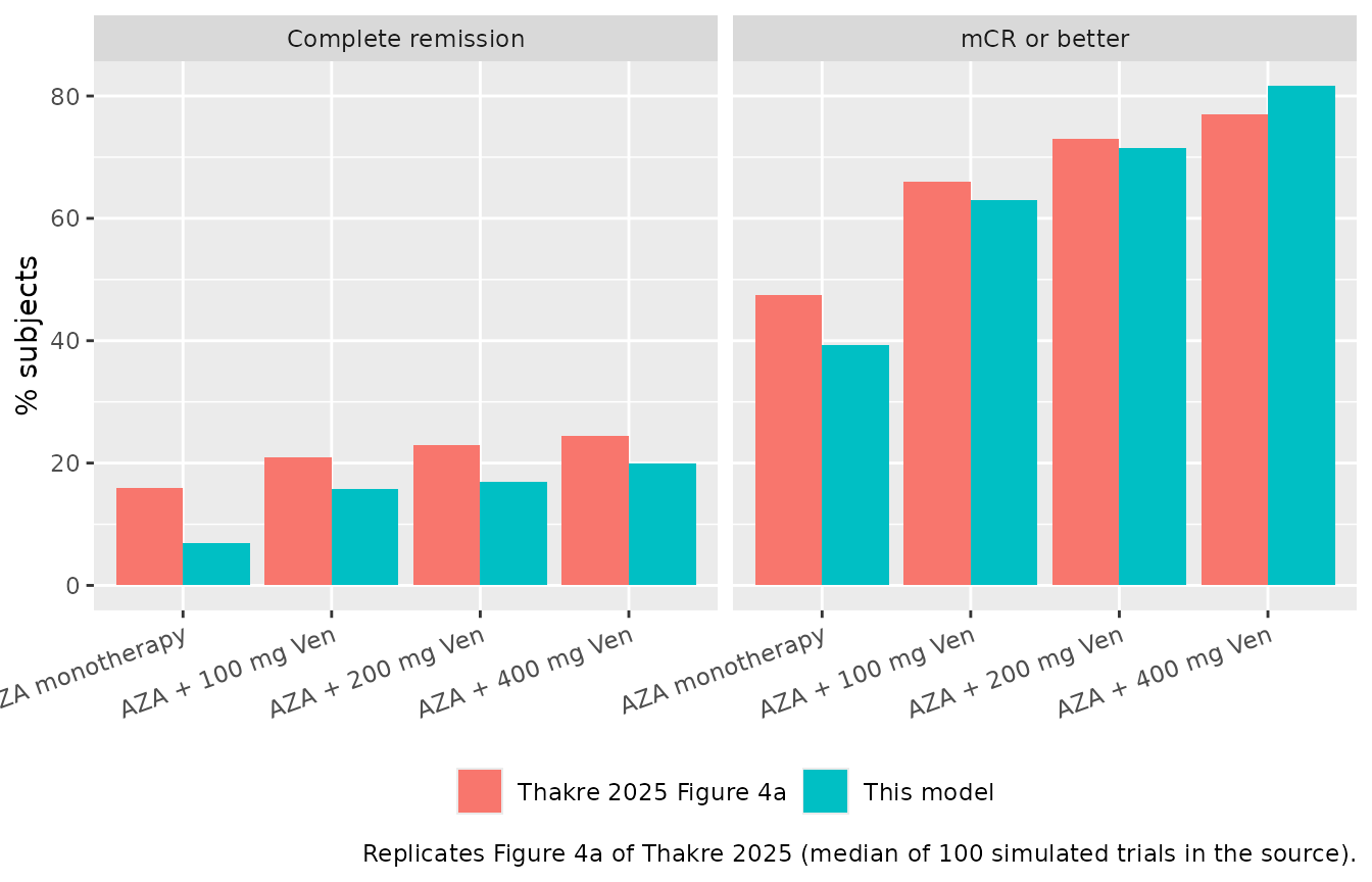
# Cohort statistics with up to 150 patients per arm (binomial SE about 4
# points).
# The bounds also absorb the diagonal-only IIV and the parametric baseline
# distributions used here (see Assumptions). A wrong slope, a wrong
# azacitidine multiplier or a units error on the venetoclax concentration
# moves these rates by tens of points.
stopifnot(
  nrow(resp_cmp) == 4,
  all(abs(resp_cmp$mCR - resp_cmp$mCR_paper) < 18),
  all(abs(resp_cmp$CR - resp_cmp$CR_paper) < 15),
  resp_cmp$mCR[resp_cmp$arm == "AZA + 400 mg Ven"] -
    resp_cmp$mCR[resp_cmp$arm == "AZA monotherapy"] > 10
)
Figure 4b: recovered blasts, grade 3+ thrombocytopenia and neutropenia
Percent of patients over time with bone-marrow blasts < 5%, platelets < 50 x 10^9/L and neutrophils < 1 x 10^9/L (the grade 3 thresholds of Table 3).
pct_over_time <- function(d) {
  d |>
    group_by(arm, time) |>
    summarise(`Recovered blasts (< 5%)` = 100 * mean(bmblast < 5),
              `Grade 3+ thrombocytopenia` = 100 * mean(PLT < 50),
              `Grade 3+ neutropenia` = 100 * mean(ANC < 1),
              .groups = "drop") |>
    pivot_longer(-c(arm, time))
}
sim |>
  filter(schedule == "Ven days 1-14") |>
  pct_over_time() |>
  ggplot(aes(time / cycle_len, value, colour = arm)) +
  geom_line() +
  facet_wrap(~name, ncol = 1) +
  scale_y_continuous(limits = c(0, 100)) +
  labs(x = "Cycle", y = "% subjects", colour = NULL,
       caption = "Replicates Figure 4b of Thakre 2025 (venetoclax days 1-14 of each cycle).") +
  theme(legend.position = "bottom")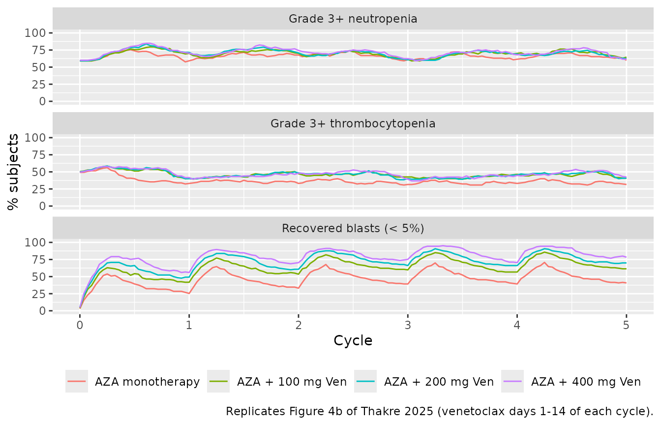
Figure 4c: grade 3+ neutropenia with continuous venetoclax
Under the original protocol venetoclax was given daily for all 28 days of each cycle. The source contrasts this with the 14-day schedule to show how the dosing holiday lowers the probability of grade 3+ neutropenia.
# The same 50 patients on both schedules: the comparison is paired.
neut_sched <- sim |>
  left_join(subjects |> select(id, k), by = "id") |>
  filter(k <= n_pat_4c) |>
  group_by(arm, schedule, time) |>
  summarise(pct = 100 * mean(ANC < 1), .groups = "drop")
bind_rows(
  neut_sched |> filter(schedule == "Ven days 1-28"),
  neut_sched |> filter(arm == "AZA monotherapy")
) |>
  ggplot(aes(time / cycle_len, pct, colour = arm)) +
  geom_line() +
  scale_y_continuous(limits = c(0, 100)) +
  labs(x = "Cycle", y = "% subjects with grade 3+ neutropenia", colour = NULL,
       caption = "Replicates Figure 4c of Thakre 2025 (venetoclax days 1-28 of each cycle).") +
  theme(legend.position = "bottom")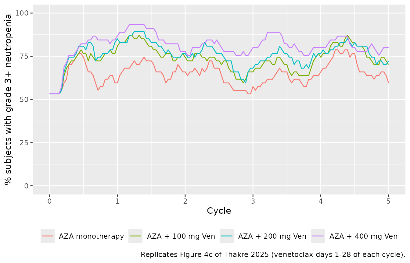
neut_cmp <- neut_sched |>
  filter(arm != "AZA monotherapy", time > 28) |>
  group_by(arm, schedule) |>
  summarise(mean_pct = mean(pct), .groups = "drop") |>
  pivot_wider(names_from = schedule, values_from = mean_pct)
knitr::kable(neut_cmp, digits = 1,
caption = "Mean % of the same 50 patients with grade 3+ neutropenia over cycles 2-5.")| arm | Ven days 1-14 | Ven days 1-28 |
|---|---|---|
| AZA + 100 mg Ven | 67.7 | 74.3 |
| AZA + 200 mg Ven | 67.6 | 76.7 |
| AZA + 400 mg Ven | 69.2 | 82.5 |
# Continuous dosing removes the 14-day recovery window, so the time-averaged
# grade 3+ neutropenia prevalence is higher. Pooled over the three doses and
# four cycles the difference (about 10-15 points) is several times its noise;
# per dose, 50 patients are too few to order the two schedules reliably.
stopifnot(
  nrow(neut_cmp) == 3,
  mean(neut_cmp$`Ven days 1-28`) - mean(neut_cmp$`Ven days 1-14`) > 3
)
Figure 2: simulated time courses by endpoint
Figure 2 is a prediction-corrected VPC against the observed study data, which cannot be reproduced without the data. The plot below shows the simulated 5th, 50th and 95th percentiles of the individual predictions (without residual error) for the 400 mg (days 1-14) regimen on the same endpoints.
sim |>
  filter(arm == "AZA + 400 mg Ven", schedule == "Ven days 1-14") |>
  select(time, `Blasts (%)` = bmblast, `Neutrophils (10^9/L)` = ANC,
         `Platelets (10^9/L)` = PLT, `RBC (10^12/L)` = RBC) |>
  pivot_longer(-time) |>
  group_by(name, time) |>
  summarise(q05 = quantile(value, 0.05), q50 = median(value), q95 = quantile(value, 0.95),
            .groups = "drop") |>
  ggplot(aes(time / cycle_len, q50)) +
  geom_ribbon(aes(ymin = q05, ymax = q95), alpha = 0.25) +
  geom_line() +
  facet_wrap(~name, scales = "free_y") +
  scale_y_log10() +
  labs(x = "Cycle", y = NULL,
       caption = "Individual predictions; compare with Figure 2 of Thakre 2025.")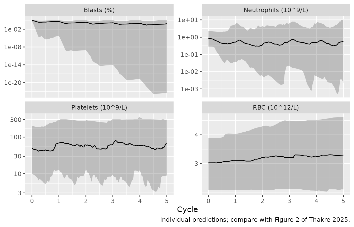
Assumptions and deviations
-
Final PD estimates come from Table 2, not from the control
stream. The
$THETAand$OMEGAvalues printed in Data S1 belong to a simulation control stream and do not match Table 2 (for exampleTHETA8= -2.80 gives kmat,P = 1.6e-3 /day against 2.02e-5 /day in Table 2). Table 2, which also reports standard errors and confidence intervals, is used for every value; the control stream supplies the structure and the fixed constants. - IIV without correlations. Table 2 reports only the diagonal of the PD IIV. The Data S1 control stream has a full block, but its values are not the final ones, so the model carries independent etas. Correlated parameters in the source (e.g. the maturation rates and the precursor elimination rates) partly offset each other there; independent etas widen the simulated spread. This, and the parametric baseline distributions, are the likely reasons the simulated CR rates sit a few points below Figure 4a.
- IIV scale. The %CV in Table 2 is inverted with the footnote formula on the base-10 ETA scale (see Source trace) and converted to the natural-log scale. The resulting variances are large (for example kmat,N 169 %CV gives a natural-log variance of 7.2), as in the source. A few percent of virtual patients draw a very stiff lineage that the solver cannot integrate through the azacitidine on/off step; they are excluded and counted above, which slightly favours the better-behaved parameter combinations.
- Azacitidine effect parameters are the multipliers on proliferation (see Source trace for the confidence-interval check that identifies them).
- PK residual error. Table S1 prints 0.222 and 3.07e-7; both match the legacy-model variances (Samineni 2022: sigma^2 0.22 and 3.07e-7), so they are treated as variances and the model stores their square roots.
-
Covariates outside Table S1. The OATP1B3 inhibitor
effect (x 0.853 on CL/F) appears only in the control stream; the Methods
state that all legacy covariate effects were retained. The orientation
of the healthy-vs-patient (1.70 for patients) and sex (0.689 for women)
effects follows the legacy model as encoded in
Samineni_2022_venetoclax. - Absorption lag. Table S1 lists a lag time (0.0533 day) without saying whether it applies to fed doses only; the model applies it to every dose. The source’s PD simulation code uses individual PK parameters and no lag.
-
Peripheral blasts. The source code declares a
peripheral-blast compartment with
DADT(6) = 0that nothing reads; it is omitted. -
Venetoclax concentration units. The PD slopes are
per mg/L of venetoclax (doses in mg, volumes in L), the units in which
A(2)/V2is computed in the source; a per-ng/mL slope would multiply the effect a thousand-fold. -
Red blood cell covariate. The source data set
records baseline red blood cells in 10^9/L (Table 1); the model takes
RBC_BASEin 10^12/L and multiplies by 1000. - Response assessment. CR and mCR are evaluated at the end of each of the five simulated cycles; the study assessed the marrow at the end of cycles 1, 2 and 4 and then every three cycles.