Magnesium sulfate (Deng 2024)
Source:vignettes/articles/Deng_2024_magnesiumSulfate.Rmd
Deng_2024_magnesiumSulfate.RmdModel and source
- Citation: Deng J, Peng L, Wang Y, Li J, Tang L, Yu Y. Population pharmacokinetics and dose optimization of magnesium sulfate in Chinese preeclampsia population. BMC Pregnancy Childbirth 2024;24:424. doi:10.1186/s12884-024-06620-x
- Description: One-compartment population PK model of magnesium sulfate (MgSO4-7H2O) given by intravenous infusion, with creatinine clearance, body mass index and concomitant furosemide effects on clearance and a concomitant furosemide effect on volume, in Chinese women with preeclampsia (Deng 2024).
- Article: https://doi.org/10.1186/s12884-024-06620-x
Deng 2024 is a prospective observational population-PK study of
intravenous magnesium sulfate for seizure prophylaxis in Chinese women
with preeclampsia. It is the third magnesium sulfate popPK model in this
library, alongside Salinger_2013_magnesiumSulfate (Indian
cohort, intramuscular and intravenous maintenance) and
Easterling_2018_magnesium_sulfate (Egyptian cohort,
continuous infusion versus serial bolus). Its distinguishing
contribution is the covariate model: creatinine clearance, body mass
index and concomitant furosemide on clearance, plus
furosemide on volume. The paper presents the furosemide effect as the
first such report for magnesium.
Read the Assumptions and deviations section before using this model. Two features of the source publication required documented interpretation: the normalising constants printed in the paper’s covariate equation are not usable as printed, and the published model carries no endogenous magnesium baseline even though the data it was fit to are total serum magnesium.
Population
pop <- rxode2::rxode(readModelDb("Deng_2024_magnesiumSulfate"))$population
str(pop, max.level = 1)
#> List of 12
#>  $ species       : chr "human"
#>  $ n_subjects    : int 51
#>  $ n_studies     : int 1
#>  $ age_range     : chr "18-45 years by inclusion criteria; observed median 31 (IQR 28-35), mean 31.86 +/- 5.22 years"
#>  $ age_median    : chr "31 years"
#>  $ weight_range  : chr "not reported; body size is characterised by BMI only (median 29.13 kg/m^2, IQR 27.16-33.30)"
#>  $ sex_female_pct: num 100
#>  $ race_ethnicity: chr "Chinese (women enrolled at the Affiliated Suzhou Hospital of Nanjing Medical University, Suzhou, Jiangsu)"
#>  $ disease_state : chr "Preeclampsia requiring intravenous MgSO4 for seizure prophylaxis; gestational age 32.31 +/- 3.92 weeks at treat"| __truncated__
#>  $ dose_range    : chr "Day 1: 5 g MgSO4-7H2O intravenous loading dose over 30-120 min followed by a 10 g maintenance dose over 6-8 h b"| __truncated__
#>  $ regions       : chr "China (Suzhou, Jiangsu)"
#>  $ notes         : chr "Prospective observational study, April 2021 - April 2023; 199 serum magnesium concentrations from 51 women (2-4"| __truncated__
51 women contributed 199 serum magnesium concentrations (two to four samples each) between April 2021 and April 2023 at the Affiliated Suzhou Hospital of Nanjing Medical University. Baseline characteristics are Deng 2024 Table 1:
| Characteristic | Value |
|---|---|
| Age (years) | 31 (28, 35); mean 31.86 +/- 5.22 |
| Gestational age (weeks) | 32.31 +/- 3.92 |
| BMI (kg/m^2) | 29.13 (27.16, 33.30) |
| Baseline magnesium (mmol/L) | 0.76 (0.71, 0.86) |
| Creatinine clearance (mL/min) | 182.18 +/- 67.15 |
| Albumin (g/L) | 30.45 +/- 4.66 |
| Calcium (tabulated as g/L) | 2.17 +/- 0.15 |
| Twin pregnancy | 4 (7.84%) |
| Labetalol | 50 (98.03%) |
| Nifedipine | 22 (43.14%) |
| Furosemide | 16 (31.37%) |
| Any adverse reaction | 21 (41.18%) |
The cohort is renally hyperfiltrating: a mean creatinine clearance of
182 mL/min reflects the 40-65% pregnancy-associated rise in glomerular
filtration rate the paper describes. Any user applying this model
outside a comparable pregnant population is extrapolating the
(CRCL/175)^0.39 term well below the range in which it was
estimated.
Dosing in the study was 5 g MgSO4-7H2O intravenously over 30-120 min on day 1 followed by a 10 g maintenance infusion over 6-8 h, then the 10 g maintenance dose alone on days 2-5. All modelled samples were drawn on day 2, after a maintenance dose with no same-day loading dose.
Unit conventions
Two conversions are load-bearing and are worth stating explicitly because the paper leaves both implicit.
Salt basis. Doses are prescribed in grams of magnesium sulfate. Following the two sibling models in this library, the salt is taken to be the heptahydrate MgSO4-7H2O (MW 246.47) used in obstetric practice, and doses are expressed in this model as mg of elemental magnesium (MW 24.305).
Concentration. Deng 2024 Figure 3 labels its visual-predictive-check y-axis “Prediction-corrected concentrations (mg/L)”, with observations spanning roughly 20-52 mg/L. That fixes the concentration unit as mg/L of elemental magnesium, and therefore fixes the additive residual SD of 3.65 as 3.65 mg/L (about 7-18% of the observed concentration range, a reasonable magnitude for a clinical-chemistry assay). Table 1 and Figure 4 report magnesium in mmol/L; 1 mmol/L = 24.305 mg/L.
MG_MW      <- 24.305                    # elemental Mg, g/mol
MGSO4_MW   <- 246.47                    # MgSO4-7H2O, g/mol
MG_PER_G   <- MG_MW / MGSO4_MW * 1000   # mg elemental Mg per g MgSO4-7H2O
BASELINE   <- 0.76 * MG_MW              # reported baseline magnesium, mg/L

c(mg_Mg_per_g_salt = MG_PER_G,
  g5  = 5  * MG_PER_G,
  g10 = 10 * MG_PER_G,
  g15 = 15 * MG_PER_G,
  baseline_mgL = BASELINE)
#> mg_Mg_per_g_salt               g5              g10              g15
#>         98.61241        493.06204        986.12407       1479.18611
#>     baseline_mgL
#>         18.47180
Source trace
Every ini() value and every model()
equation, with its origin in the source publication. In-file comments
next to each ini() entry carry the same information.
| Model quantity | Value | Source location |
|---|---|---|
lcl (CL) |
2.98 L/h | Table 2, tvCL; 95% CI 1.29-4.62. Also Abstract and
Discussion. |
lvc (V) |
25.07 L | Table 2, tvV; 95% CI 23.31-26.82 |
e_crcl_cl |
+0.39 | Table 2, dCLdCCR; 95% CI 0.31-0.46 |
e_bmi_cl |
-0.54 | Table 2, dCLdBMI; 95% CI (-0.70)-(-0.38) |
e_conmed_furosemide_cl |
-0.16 | Table 2, dCLdfurosemide; 95% CI (-0.22)-(-0.096) |
e_conmed_furosemide_vc |
-0.25 | Table 2, dVdfurosemide; 95% CI (-0.34)-(-0.16) |
etalcl |
0.082 (variance) | Table 2, omega^2 CL; shrinkage 13.05% |
etalvc |
0.023 (variance) | Table 2, omega^2 V; shrinkage 13.04% |
addSd |
3.65 mg/L | Table 2, stdev0; 95% CI 3.20-4.09 |
| CL equation form | power CRCL, power BMI, fractional furosemide,
exp(eta)
|
Results, “The equations for V and CL were as follows” |
| V equation form | fractional furosemide, exp(eta)
|
Results, same equation block |
| One-compartment disposition | – | Results, “adequately described by one-compartment structural model” |
| Additive residual error | – | Results, “an additive error model was used to evaluate the residual variability” |
| CRCL reference 175 mL/min | deviation | Monte Carlo section, “CCR and BMI are taken at the median (CCR:175 ml/min, BMI:29 kg/m2)”. NOT the printed constant – see Assumptions and deviations. |
| BMI reference 29 kg/m^2 | deviation | Monte Carlo section, same sentence. NOT the printed constant. |
| Concentration unit mg/L | – | Figure 3 y-axis |
| Baseline magnesium 0.76 mmol/L | not a model parameter | Table 1 and Results; see Assumptions and deviations |
Virtual cohort
Two arms of 100 women each, matching the covariate distributions in Table 1, split by furosemide use. Creatinine clearance is drawn log-normally with the Table 1 mean and SD; BMI is drawn log-normally from the Table 1 median and interquartile range.
rxode2::rxSetSeed(20240424)
set.seed(20240424)

n_arm <- 100L

# CRCL: mean 182.18, SD 67.15 (Table 1) matched on the log scale
crcl_cv     <- 67.15 / 182.18
crcl_sdlog  <- sqrt(log(1 + crcl_cv^2))
crcl_meanlog <- log(182.18) - crcl_sdlog^2 / 2

# BMI: median 29.13, IQR 27.16-33.30 (Table 1)
bmi_sdlog   <- log(33.30 / 27.16) / (2 * qnorm(0.75))
bmi_meanlog <- log(29.13)

make_arm <- function(furo, offset) {
  data.frame(
    id                = offset + seq_len(n_arm),
    CRCL              = rlnorm(n_arm, crcl_meanlog, crcl_sdlog),
    BMI               = rlnorm(n_arm, bmi_meanlog, bmi_sdlog),
    CONMED_FUROSEMIDE = furo,
    arm               = if (furo == 1) "Furosemide" else "No furosemide"
  )
}

cohort <- dplyr::bind_rows(make_arm(0, 0L), make_arm(1, n_arm))

cohort |>
  dplyr::group_by(arm) |>
  dplyr::summarise(n = dplyr::n(),
                   CRCL_median = median(CRCL), CRCL_mean = mean(CRCL),
                   CRCL_sd = sd(CRCL), BMI_median = median(BMI),
                   .groups = "drop") |>
  knitr::kable(digits = 2,
caption = "Simulated covariate distributions against Table 1 targets (CRCL mean 182.18 +/- 67.15 mL/min; BMI median 29.13 kg/m^2).")| arm | n | CRCL_median | CRCL_mean | CRCL_sd | BMI_median |
|---|---|---|---|---|---|
| Furosemide | 100 | 174.71 | 198.02 | 82.48 | 29.21 |
| No furosemide | 100 | 157.41 | 177.20 | 77.14 | 29.43 |
The regimen simulated below is the one Deng 2024 recommends for women not receiving furosemide and reports in Figure 4 and Figure 5 panel (d): a 5 g loading dose over 20 minutes followed by a 10 g maintenance dose over 6.7 h. Observations run to 24 h so that the terminal phase is well characterised for non-compartmental analysis.
T_LOAD  <- 20 / 60      # 20 min loading infusion
T_MAINT <- 6.7          # 6.7 h maintenance infusion
AMT_LOAD  <- 5  * MG_PER_G
AMT_MAINT <- 10 * MG_PER_G
T_END <- T_LOAD + T_MAINT

times_obs <- sort(unique(c(
  seq(0, 1, by = 0.05),
  seq(1.25, 8, by = 0.25),
  T_LOAD, T_END,
  seq(8.5, 24, by = 0.5)
)))

obs_rows <- cohort |>
  tidyr::expand_grid(time = times_obs) |>
  dplyr::mutate(evid = 0L, amt = 0, dur = 0, cmt = "central")

dose_rows <- dplyr::bind_rows(
  cohort |> dplyr::mutate(time = 0,      evid = 1L, amt = AMT_LOAD,  dur = T_LOAD,  cmt = "central"),
  cohort |> dplyr::mutate(time = T_LOAD, evid = 1L, amt = AMT_MAINT, dur = T_MAINT, cmt = "central")
)

events <- dplyr::bind_rows(obs_rows, dose_rows) |>
  dplyr::arrange(id, time, dplyr::desc(evid))

stopifnot(
  !anyDuplicated(events[events$evid == 1L, c("id", "time")]),
  all(c("CRCL", "BMI", "CONMED_FUROSEMIDE") %in% names(events))
)
Simulation
rxSolve() on an rxUi object scales
super-linearly in the number of subjects, so each arm is solved in its
own call.
mod <- readModelDb("Deng_2024_magnesiumSulfate")

solve_arm <- function(model, arm_name) {
  ev <- events[events$arm == arm_name, ]
  rxode2::rxSolve(model, events = ev,
                  keep = c("CRCL", "BMI", "CONMED_FUROSEMIDE", "arm"),
                  returnType = "data.frame")
}

# Typical-value predictions: zeroRe() removes both IIV and residual error.
mod_typ <- rxode2::zeroRe(mod)
sim_typ <- dplyr::bind_rows(
  solve_arm(mod_typ, "No furosemide"),
  solve_arm(mod_typ, "Furosemide")
)
#> ℹ omega/sigma items treated as zero: 'etalvc', 'etalcl'
#> Warning: multi-subject simulation without without 'omega'
#> ℹ omega/sigma items treated as zero: 'etalvc', 'etalcl'
#> Warning: multi-subject simulation without without 'omega'

# Stochastic cohort: IIV retained, residual error suppressed so that Cc is the
# individual prediction.
rxode2::rxSetSeed(20240424)
mod_iiv <- rxode2::zeroRe(mod, which = "sigma")
sim_iiv <- dplyr::bind_rows(
  solve_arm(mod_iiv, "No furosemide"),
  solve_arm(mod_iiv, "Furosemide")
)

nrow(sim_typ)
#> [1] 16600
Verification gate 1: closed-form solution
The model is a one-compartment system receiving two sequential
zero-order infusions, so it has a closed-form solution. Comparing the
rxode2 solve against that solution for the reference
subject (CRCL 175 mL/min, BMI 29 kg/m^2, no furosemide) tests the
implementation with no confounding from covariates or random effects.
Both sides use the same parameter values, so the only difference is
integrator error and the tolerance is set accordingly.
CL_REF <- 2.98
V_REF  <- 25.07
K_REF  <- CL_REF / V_REF

conc_two_infusions <- function(t, cl, v, amt_load, t_load, amt_maint, t_maint) {
  k  <- cl / v
  rL <- amt_load / t_load
  rM <- amt_maint / t_maint
  c_load_end  <- (rL / cl) * (1 - exp(-k * t_load))
  c_maint_end <- (rM / cl) * (1 - exp(-k * t_maint)) + c_load_end * exp(-k * t_maint)
  ifelse(
    t <= t_load,
    (rL / cl) * (1 - exp(-k * t)),
    ifelse(
      t <= t_load + t_maint,
      (rM / cl) * (1 - exp(-k * (t - t_load))) + c_load_end * exp(-k * (t - t_load)),
      c_maint_end * exp(-k * (t - t_load - t_maint))
    )
  )
}

ref_ev <- rxode2::et(amt = AMT_LOAD,  dur = T_LOAD,  cmt = "central", time = 0) |>
  rxode2::et(amt = AMT_MAINT, dur = T_MAINT, cmt = "central", time = T_LOAD) |>
  rxode2::et(times_obs, cmt = "central") |>
  as.data.frame()
ref_ev$id <- 1L
ref_ev$CRCL <- 175
ref_ev$BMI <- 29
ref_ev$CONMED_FUROSEMIDE <- 0

ref_sim <- rxode2::rxSolve(mod_typ, ref_ev, returnType = "data.frame")
#> ℹ omega/sigma items treated as zero: 'etalvc', 'etalcl'
ref_obs <- ref_sim[!is.na(ref_sim$Cc), ]
ref_obs$analytic <- conc_two_infusions(
  ref_obs$time, CL_REF, V_REF, AMT_LOAD, T_LOAD, AMT_MAINT, T_MAINT
)

closed_form_err <- max(abs(ref_obs$Cc - ref_obs$analytic) /
                         pmax(ref_obs$analytic, 1e-8))
closed_form_err
#> [1] 9.734301e-07

# Same parameters on both sides: this is pure numerical error, so assert tightly.
stopifnot(closed_form_err < 1e-6)
The reference subject’s clearance and volume must also come back exactly as Table 2 reports them, confirming that the covariate term is 1 at the reference covariate values.
Verification gate 2: covariate model
Each covariate term is checked against the printed equation
independently. (CRCL/175)^0.39, (BMI/29)^-0.54
and the two furosemide fractional-change terms are all deterministic
functions of the covariate vector, so exact agreement is required.
expected_cl <- function(crcl, bmi, furo) {
  CL_REF * (crcl / 175)^0.39 * (bmi / 29)^(-0.54) * (1 - 0.16 * furo)
}
expected_vc <- function(furo) V_REF * (1 - 0.25 * furo)

cov_check <- sim_typ |>
  dplyr::distinct(id, arm, CRCL, BMI, CONMED_FUROSEMIDE, cl, vc) |>
  dplyr::mutate(
    cl_expected = expected_cl(CRCL, BMI, CONMED_FUROSEMIDE),
    vc_expected = expected_vc(CONMED_FUROSEMIDE),
    cl_err = abs(cl - cl_expected) / cl_expected,
    vc_err = abs(vc - vc_expected) / vc_expected
  )

c(max_cl_err = max(cov_check$cl_err), max_vc_err = max(cov_check$vc_err))
#>   max_cl_err   max_vc_err
#> 3.405808e-15 2.078439e-15

stopifnot(max(cov_check$cl_err) < 1e-10, max(cov_check$vc_err) < 1e-10)
The furosemide effect must reproduce the Table 2 multipliers of 0.84 on clearance and 0.75 on volume exactly.
furo_ratio <- cov_check |>
  dplyr::group_by(CONMED_FUROSEMIDE) |>
  dplyr::summarise(vc = unique(round(vc, 8)), .groups = "drop")

vc_ratio <- furo_ratio$vc[furo_ratio$CONMED_FUROSEMIDE == 1] /
  furo_ratio$vc[furo_ratio$CONMED_FUROSEMIDE == 0]

# Clearance ratio at matched covariates, isolating the furosemide term.
cl_ratio <- expected_cl(175, 29, 1) / expected_cl(175, 29, 0)

c(vc_ratio = vc_ratio, cl_ratio = cl_ratio)
#> vc_ratio cl_ratio
#>     0.75     0.84

stopifnot(abs(vc_ratio - 0.75) < 1e-8, abs(cl_ratio - 0.84) < 1e-8)
Both effects lower the parameter and therefore raise serum magnesium, matching the paper’s statement that “patients received furosemide had higher blood magnesium concentrations than those who did not receive furosemide”.
Replicate published figures
Figure 4: median concentration-time profiles
Figure 4 of Deng 2024 plots the median simulated magnesium concentration against time for eight dosing regimens at median covariates, split by furosemide use. Below we reproduce the two 10 g maintenance regimens for both arms, on the paper’s mmol/L axis and with the reported endogenous baseline added so the curves are on the same footing as the published ones.
fig4 <- sim_typ |>
  dplyr::filter(!is.na(Cc), time <= 8) |>
  dplyr::group_by(arm, time) |>
  dplyr::summarise(mmol = (median(Cc) + BASELINE) / MG_MW, .groups = "drop")

ggplot(fig4, aes(time, mmol, colour = arm)) +
  geom_line(linewidth = 0.8) +
  geom_hline(yintercept = c(2, 3.5), linetype = "dashed", colour = "grey40") +
  scale_x_continuous(breaks = 0:8) +
  labs(x = "Time (hours)", y = "Magnesium concentration (mmol/L)",
       colour = NULL,
       title = "Figure 4 (replicated): 5 g load + 10 g maintenance",
       caption = paste("Dashed lines: the 2.0-3.5 mmol/L therapeutic window.",
                       "Endogenous baseline of 0.76 mmol/L added; see Assumptions.")) +
  theme(legend.position = "bottom")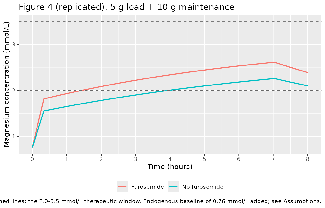
The published curves for these two regimens read as follows at integer hours (Figure 4, grey series). We compare them against the replication.
published_fig4 <- tibble::tibble(
  time = 0:8,
  `No furosemide` = c(0.80, 2.08, 2.30, 2.49, 2.65, 2.77, 2.89, 2.99, 2.53),
  `Furosemide`    = c(0.80, 2.64, 2.89, 3.09, 3.27, 3.42, 3.53, 3.62, 3.01)
) |>
  tidyr::pivot_longer(-time, names_to = "arm", values_to = "published")

fig4_cmp <- sim_typ |>
  dplyr::filter(!is.na(Cc), time %in% 0:8) |>
  dplyr::group_by(arm, time) |>
  dplyr::summarise(modelled = (median(Cc) + BASELINE) / MG_MW, .groups = "drop") |>
  dplyr::inner_join(published_fig4, by = c("arm", "time")) |>
  dplyr::mutate(ratio_drug = (modelled - 0.76) / (published - 0.76))

fig4_cmp |>
  dplyr::filter(time > 0) |>
  dplyr::select(arm, time, modelled, published, ratio_drug) |>
  dplyr::rename("Arm" = arm, "Time (h)" = time,
                "Modelled (mmol/L)" = modelled,
                "Published (mmol/L)" = published,
                "Modelled/published, drug only" = ratio_drug) |>
  knitr::kable(digits = 3,
caption = "Replication of Deng 2024 Figure 4 at integer hours. The last column divides the baseline-subtracted concentrations.")| Arm | Time (h) | Modelled (mmol/L) | Published (mmol/L) | Modelled/published, drug only |
|---|---|---|---|---|
| Furosemide | 1 | 1.930 | 2.64 | 0.622 |
| Furosemide | 2 | 2.084 | 2.89 | 0.622 |
| Furosemide | 3 | 2.219 | 3.09 | 0.626 |
| Furosemide | 4 | 2.337 | 3.27 | 0.628 |
| Furosemide | 5 | 2.440 | 3.42 | 0.632 |
| Furosemide | 6 | 2.531 | 3.53 | 0.639 |
| Furosemide | 7 | 2.609 | 3.62 | 0.647 |
| Furosemide | 8 | 2.386 | 3.01 | 0.723 |
| No furosemide | 1 | 1.650 | 2.08 | 0.675 |
| No furosemide | 2 | 1.782 | 2.30 | 0.664 |
| No furosemide | 3 | 1.899 | 2.49 | 0.659 |
| No furosemide | 4 | 2.004 | 2.65 | 0.658 |
| No furosemide | 5 | 2.097 | 2.77 | 0.665 |
| No furosemide | 6 | 2.181 | 2.89 | 0.667 |
| No furosemide | 7 | 2.255 | 2.99 | 0.670 |
| No furosemide | 8 | 2.100 | 2.53 | 0.757 |
The modelled curve sits systematically below the published one by a near-constant factor on the drug-attributable concentration. That factor is reported rather than corrected; see Assumptions and deviations, which shows that the discrepancy is in amplitude only and not in shape.
Figure 4 shape: the diagnostic that fixes CL/V
Because the amplitude of Figure 4 is not reproducible, the useful
information in it is its shape. If the modelled and published
profiles differ only by a constant scale factor, then the ratio
modelled / published of the baseline-subtracted
concentrations is flat across time, and the elimination rate constant
k = CL/V is right even though the amplitude is not. If
k is wrong, that ratio drifts systematically.
Using all seven hourly points makes this robust to the roughly +/-
0.02 mmol/L uncertainty of reading values off a raster figure. (A
curvature statistic built from differences between adjacent points – for
example (C7-C5)/(C5-C3) – is not robust: the
differences involved are only 0.2-0.3 mmol/L, so a 0.02 mmol/L reading
error moves the statistic by more than 0.1 and the two arms give
conflicting answers. It is not used here.)
cl_as_printed <- 2.98 * (175 / 51)^0.39 * (29 / 51)^(-0.54)

shape_ratio <- function(cl, vc, published_drug) {
  modelled <- conc_two_infusions(1:7, cl, vc,
                                 AMT_LOAD, T_LOAD, AMT_MAINT, T_MAINT) / MG_MW
  modelled / published_drug
}

shape_one_arm <- function(a) {
  furo <- as.integer(a == "Furosemide")
  pub  <- published_fig4$published[published_fig4$arm == a &
                                     published_fig4$time %in% 1:7] - 0.76
  vc   <- V_REF * (1 - 0.25 * furo)
  impl <- shape_ratio(2.98          * (1 - 0.16 * furo), vc, pub)
  litl <- shape_ratio(cl_as_printed * (1 - 0.16 * furo), vc, pub)
  data.frame(
    arm = a,
    implemented_mean = mean(impl), implemented_cv = 100 * sd(impl) / mean(impl),
    as_printed_mean  = mean(litl), as_printed_cv  = 100 * sd(litl) / mean(litl)
  )
}

shape_tbl <- dplyr::bind_rows(lapply(c("No furosemide", "Furosemide"),
                                     shape_one_arm))

shape_tbl |>
  dplyr::rename("Arm" = arm,
                "Ratio, implemented" = implemented_mean,
                "CV%, implemented"   = implemented_cv,
                "Ratio, as printed"  = as_printed_mean,
                "CV%, as printed"    = as_printed_cv) |>
  knitr::kable(digits = c(0, 3, 1, 3, 1),
caption = "Modelled/published ratio of drug-attributable concentration at t = 1-7 h. A flat ratio (low CV%) means the shape matches and only the amplitude differs.")| Arm | Ratio, implemented | CV%, implemented | Ratio, as printed | CV%, as printed |
|---|---|---|---|---|
| No furosemide | 0.659 | 1.0 | 0.479 | 15.0 |
| Furosemide | 0.633 | 1.6 | 0.446 | 13.9 |
c(cl_if_equation_read_literally = cl_as_printed)
#> cl_if_equation_read_literally
#>                      6.537952

# The implemented reading differs from Figure 4 by a near-constant factor in
# both arms; the literal reading of the printed equation drifts monotonically.
stopifnot(
  all(shape_tbl$implemented_cv < 4),
  all(shape_tbl$as_printed_cv > 3 * shape_tbl$implemented_cv)
)
Under the implemented reading the ratio is flat to within 1-2% in both arms, so Figure 4 and this model agree on shape and disagree only on scale. Under the literal reading of the printed equation the ratio falls monotonically from about 0.61 to 0.40 across the same seven hours, a roughly ten-fold worse agreement. This is the quantitative basis for the covariate-reference decision documented below.
Stochastic cohort profile
band <- sim_iiv |>
  dplyr::filter(!is.na(Cc), time <= 16) |>
  dplyr::group_by(arm, time) |>
  dplyr::summarise(
    med = (median(Cc) + BASELINE) / MG_MW,
    lo  = (quantile(Cc, 0.05) + BASELINE) / MG_MW,
    hi  = (quantile(Cc, 0.95) + BASELINE) / MG_MW,
    .groups = "drop"
  )

ggplot(band, aes(time, med)) +
  geom_ribbon(aes(ymin = lo, ymax = hi), alpha = 0.25) +
  geom_line(linewidth = 0.8) +
  geom_hline(yintercept = c(2, 3.5), linetype = "dashed", colour = "grey40") +
  facet_wrap(~ arm) +
  labs(x = "Time (hours)", y = "Magnesium concentration (mmol/L)",
       title = "Simulated cohort, 5 g load + 10 g maintenance",
       caption = "Line = median; ribbon = 5th-95th centile across 100 women per arm.")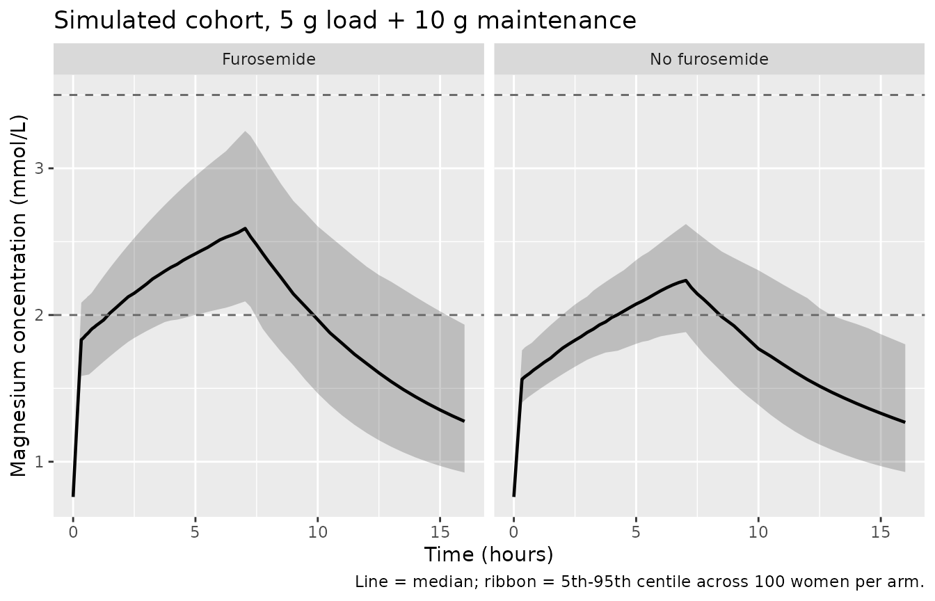
PKNCA validation
Non-compartmental analysis of the typical-value profiles. Because the
model predicts administered magnesium only, no baseline correction is
needed before NCA. For a linear one-compartment model the NCA-derived
clearance (Dose / AUC_inf) and half-life must recover the
model’s own CL and ln(2) * V / CL exactly,
which makes this a strict check of the packaged parameters rather than a
descriptive summary.
conc_nca <- sim_typ |>
  dplyr::filter(!is.na(Cc)) |>
  dplyr::select(id, time, Cc, arm)

# Time-zero records are present by construction (times_obs starts at 0), which
# keeps PKNCA from warning about an AUC interval starting before the first
# measurement.
stopifnot(all(tapply(conc_nca$time, conc_nca$id, min) == 0))

dose_nca <- events |>
  dplyr::filter(evid == 1L) |>
  dplyr::group_by(id, arm) |>
  dplyr::summarise(time = min(time), amt = sum(amt), .groups = "drop")

conc_obj <- PKNCA::PKNCAconc(conc_nca, Cc ~ time | arm + id,
                             concu = "mg/L", timeu = "h")
dose_obj <- PKNCA::PKNCAdose(dose_nca, amt ~ time | arm + id, doseu = "mg")

intervals <- data.frame(
  start       = 0,
  end         = Inf,
  cmax        = TRUE,
  tmax        = TRUE,
  auclast     = TRUE,
  aucinf.obs  = TRUE,
  half.life   = TRUE,
  cl.obs      = TRUE
)

nca_res <- PKNCA::pk.nca(
  PKNCA::PKNCAdata(conc_obj, dose_obj, intervals = intervals)
)

nca_wide <- as.data.frame(nca_res) |>
  dplyr::select(arm, id, PPTESTCD, PPORRES) |>
  tidyr::pivot_wider(names_from = PPTESTCD, values_from = PPORRES)

nca_wide |>
  dplyr::group_by(arm) |>
  dplyr::summarise(
    Cmax      = median(cmax),
    Tmax      = median(tmax),
    AUClast   = median(auclast),
    AUCinf    = median(aucinf.obs),
    half_life = median(half.life),
    CL_nca    = median(cl.obs),
    .groups   = "drop"
  ) |>
  dplyr::rename("Arm" = arm, "Cmax (mg/L)" = Cmax, "Tmax (h)" = Tmax,
                "AUClast (mg*h/L)" = AUClast, "AUCinf (mg*h/L)" = AUCinf,
                "t1/2 (h)" = half_life, "CL from NCA (L/h)" = CL_nca) |>
  knitr::kable(digits = 3,
caption = "PKNCA results on the typical-value profiles, by arm.")| Arm | Cmax (mg/L) | Tmax (h) | AUClast (mg*h/L) | AUCinf (mg*h/L) | t1/2 (h) | CL from NCA (L/h) |
|---|---|---|---|---|---|---|
| Furosemide | 45.010 | 7.033 | 551.380 | 585.694 | 5.161 | 2.526 |
| No furosemide | 36.386 | 7.033 | 468.818 | 514.036 | 6.039 | 2.878 |
Comparison against the model’s own parameters
nca_gate <- nca_wide |>
  dplyr::inner_join(
    sim_typ |> dplyr::distinct(id, cl, vc),
    by = "id"
  ) |>
  dplyr::mutate(
    cl_expected = cl,
    hl_expected = log(2) * vc / cl,
    cl_pct_diff = 100 * (cl.obs - cl_expected) / cl_expected,
    hl_pct_diff = 100 * (half.life - hl_expected) / hl_expected
  )

nca_gate |>
  dplyr::summarise(
    max_abs_cl_pct_diff = max(abs(cl_pct_diff)),
    max_abs_hl_pct_diff = max(abs(hl_pct_diff))
  )
#> # A tibble: 1 × 2
#>   max_abs_cl_pct_diff max_abs_hl_pct_diff
#>                 <dbl>               <dbl>
#> 1             0.00247           0.0000171

# Both sides are built from the same parameter values, so the residual is
# trapezoidal / log-linear-regression error only and a tight bound is correct.
stopifnot(
  max(abs(nca_gate$cl_pct_diff)) < 1,
  max(abs(nca_gate$hl_pct_diff)) < 1
)
Deng 2024 reports no non-compartmental parameters, so there is no published NCA table to compare against; the check above therefore verifies the packaged model against its own closed-form exposure metrics. The reference subject’s values are:
Therapeutic target attainment
The paper’s clinical endpoint is the fraction of women inside the 2.0-3.5 mmol/L therapeutic window. Its own observed figure is that 5 of 51 women (9.80%) reached the window at 4-5 h on day 2, when only the 10 g maintenance dose was given and no loading dose preceded it. Simulating that day-2 regimen gives the model’s counterpart.
maint_only <- cohort |>
  tidyr::expand_grid(time = c(0, 4, 4.5, 5, 7)) |>
  dplyr::mutate(evid = 0L, amt = 0, dur = 0, cmt = "central") |>
  dplyr::bind_rows(
    cohort |> dplyr::mutate(time = 0, evid = 1L, amt = AMT_MAINT,
                            dur = 7, cmt = "central")
  ) |>
  dplyr::arrange(id, time, dplyr::desc(evid))

rxode2::rxSetSeed(20240424)
sim_maint <- dplyr::bind_rows(
  rxode2::rxSolve(mod_iiv, events = maint_only[maint_only$arm == "No furosemide", ],
                  keep = c("arm"), returnType = "data.frame"),
  rxode2::rxSolve(mod_iiv, events = maint_only[maint_only$arm == "Furosemide", ],
                  keep = c("arm"), returnType = "data.frame")
)

pta <- sim_maint |>
  dplyr::filter(!is.na(Cc), time %in% c(4, 4.5, 5)) |>
  dplyr::mutate(total_mmol = (Cc + BASELINE) / MG_MW) |>
  dplyr::group_by(arm, time) |>
  dplyr::summarise(median_mmol = median(total_mmol),
                   pct_in_window = 100 * mean(total_mmol >= 2 & total_mmol <= 3.5),
                   .groups = "drop")

pta |>
  dplyr::rename("Arm" = arm, "Time (h)" = time,
                "Median total Mg (mmol/L)" = median_mmol,
                "% in 2.0-3.5 mmol/L" = pct_in_window) |>
  knitr::kable(digits = 2,
caption = "Maintenance-dose-only day-2 regimen. Deng 2024 observed 9.80% target attainment at 4-5 h.")| Arm | Time (h) | Median total Mg (mmol/L) | % in 2.0-3.5 mmol/L |
|---|---|---|---|
| Furosemide | 4.0 | 1.69 | 1 |
| Furosemide | 4.5 | 1.78 | 8 |
| Furosemide | 5.0 | 1.85 | 23 |
| No furosemide | 4.0 | 1.49 | 0 |
| No furosemide | 4.5 | 1.57 | 0 |
| No furosemide | 5.0 | 1.63 | 1 |
The model reproduces the paper’s central clinical finding qualitatively: a maintenance dose alone leaves the typical woman well below the therapeutic window at 4-5 h, which is the observation that motivated the paper’s dose-optimisation exercise. The attained percentage is lower than the observed 9.80% for the same reason the Figure 4 amplitude is low, so this is reported as a directional check and not asserted as a numeric match.
Assumptions and deviations
1. The normalising constant in the printed clearance equation (major)
Deng 2024 prints its final covariate model in the Results section as
CL(L/h) = 2.98 x (CCR/51)^0.39 x (BMI/51)^-0.54 x (1 - 0.16 x furosemide) x exp(etaCL)
V(L)    = 25.07 x (1 - 0.25 x furosemide) x exp(etaV)
The constant 51 is used to normalise
both covariates, and 51 is the number of subjects in
the study (n = 51, Table 1 header). It is not a plausible
reference value for either covariate: creatinine clearance has a cohort
mean of 182 mL/min and BMI a median of 29 kg/m^2. This model instead
normalises by the study medians, (CRCL/175)^0.39 and
(BMI/29)^-0.54.
Four independent lines of evidence support that reading.
-
Table 2 labels 2.98 as
tvCL, with the footnote “tv, typical population value”. Read literally, the printed equation puts clearance at the study median covariates at2.98 * (175/51)^0.39 * (29/51)^-0.54 = 6.54 L/h, so 2.98 would be a bare scaling constant and not the typical value the table says it is. - The Abstract and Discussion both state the population value directly: “The population parameter estimates were as follows: CL was 2.98 L/h” and “The model estimate of the population CL was 2.98 L/h”.
- The Discussion’s literature comparison only works at 2.98. It says “Our study found the CL value of 2.98 CL/h, which is lower than the values typically described in literature”, against a quoted literature range of 1.38-5.00 L/h. A clearance of 6.54 L/h would be above that range, which would invert the sentence.
-
The paper’s own Figure 4 agrees on shape only under this
reading. The ratio of modelled to published drug-attributable
concentration across t = 1-7 h is flat under the implemented reading
(mean 0.659, CV 1.0% without furosemide; mean 0.633, CV 1.6% with),
meaning the two profiles differ by a constant factor and therefore share
the same
CL/V. Under the literal reading the same ratio drifts monotonically from 0.61 to 0.40 (CV 15% and 14%). Note that this argument establishes only thatCL/Vis right; it says nothing about the absolute scale, which Figure 4 gets wrong under either reading (see deviation 3).
The two reference values themselves come from the paper’s Monte Carlo section, which states them verbatim: “when CCR and BMI are taken at the median (CCR:175 ml/min, BMI:29 kg/m2)”. Table 1 reports the BMI median as 29.13 rather than 29; using 29.13 changes the BMI multiplier by 0.24% and is immaterial. Table 1 gives no CCR median, only the mean 182.18 +/- 67.15; using 182.18 in place of 175 changes the CCR multiplier by 1.7%.
Consequence for users. Anyone re-deriving this model
from the printed equation alone will obtain clearances 2.2-fold higher
than this implementation. The exponents, the furosemide terms,
V and the variance terms are unaffected.
2. No endogenous magnesium baseline (major)
Deng 2024 Table 2 estimates no baseline magnesium parameter, so the
packaged model predicts administered magnesium only and
Cc goes to zero after washout. The data the model was fit
to are total serum magnesium: Table 1 reports an observed baseline of
0.76 mmol/L (18.5 mg/L) and Figure 3 shows observations spanning 20-52
mg/L, none of which approach zero.
This is a genuine misspecification in the source publication rather than an extraction choice, and the paper appears to have worked around it in simulation without recording it as a parameter: every curve in Figure 4 starts at 0.80 mmol/L, which can only come from a baseline term added after the fact. The paper also notes that its conditional weighted residuals “still had an obvious trend, suggesting that there may be important factors that are not found to affect the accuracy of the model” – a missing baseline is exactly the kind of factor that produces such a trend.
The model is packaged as published. This vignette adds the reported
0.76 mmol/L baseline explicitly wherever it compares against a published
total-magnesium quantity, and users comparing against measured total
serum magnesium should add roughly 18.5 mg/L to Cc. Both
sibling models estimate a baseline directly
(Salinger_2013_magnesiumSulfate BL = 20.8 mg/L,
Easterling_2018_magnesium_sulfate BL = 22.48 mg/L), so a
user moving between the three models must handle this difference
deliberately.
3. Figure 4 amplitude is not reproducible (erratum)
With the baseline added, the replication above tracks the
shape of Figure 4 closely but sits below it by a near-constant
factor of about 0.66 (no furosemide) or 0.63 (furosemide) on the
drug-attributable concentration. Because that factor varies by only 1-2%
across seven hourly time points in both arms, the disagreement is an
amplitude effect – a dose-amount or volume scaling – and not a
structural one: a wrong CL/V would make the ratio drift
with time, as the shape test above shows it does under the alternative
reading.
Reproducing Figure 4’s amplitude with V = 25.07 L would
require the 10 g maintenance dose to deliver about 1.53 g of elemental
magnesium, whereas 10 g of MgSO4-7H2O delivers 0.986 g and 10 g of the
anhydrous salt would deliver 2.02 g; neither matches, and no
pharmaceutical hydrate of magnesium sulfate has the implied molecular
weight. The discrepancy is therefore reported and left uncorrected.
No parameter has been tuned to close it. The Table 2
estimates, which are the reusable content of the paper, reproduce their
own closed-form exposure metrics exactly (gates 1 and 2 and the PKNCA
comparison above).
4. Interpretation of the variance terms
Table 2’s inter-individual variability rows are labelled
omega^2 V and omega^2 CL and are read here as
log-scale variances (0.023 and 0.082, i.e. CV 15.3% and
29.2%). The header of the adjacent column reads “CV (%)” and gives 26.89
for V and 17.38 for CL, but those cannot be the IIV CVs: the smaller
variance would then have to carry the larger CV. They are the relative
standard errors of the variance estimates, consistent with the bootstrap
column alongside them. No eta correlation is reported, so the two random
effects are coded independently.
5. Other assumptions
- Salt basis. The paper never states whether “10 g” refers to the heptahydrate or the anhydrous salt. The heptahydrate is assumed, matching obstetric practice and both sibling models.
-
Creatinine clearance assay. The paper reports
“creatinine clearance (CCR)” without naming an estimating equation, and
does not state whether the values are body-surface-area normalised. They
are treated as raw mL/min. The
CRCLcanonical entry has ample precedent for raw un-normalised values. - Covariate distributions. Table 1 reports CRCL as a mean with SD and BMI as a median with IQR; the virtual cohort draws both log-normally to match those summaries. Body weight is never reported, so no allometric term is possible and none is in the model.
- Furosemide is confounded with disease severity. The paper attributes the furosemide effect to the volume overload and renal impairment that prompted the prescription rather than to a drug interaction. The indicator should not be transported to a population in which furosemide is given for another reason.
- Infusion durations. Study infusions ran 30-120 min (loading) and 6-8 h (maintenance) at clinician discretion. This vignette uses the 20 min and 6.7 h durations of the paper’s own Monte Carlo regimens so the replication is comparable to Figure 4.
-
Screened but not retained. Age, serum albumin,
calcium, labetalol, nifedipine, adverse-reaction occurrence, gestational
age, diagnosis and mode of delivery were all screened by the stepwise
covariate model and rejected; no point estimates are reported for any of
them. Age and albumin are recorded in the model file’s
covariatesDataExcludedfor provenance. - Calcium units. Table 1 tabulates calcium as “2.17 +/- 0.15 g/L”, which is almost certainly mmol/L. Calcium is not in the model, so nothing depends on it.
- No external validation. The paper states that the model was only internally evaluated.