Automated popPK model search: ribociclib, camizestrant, osimertinib, olaparib, tezepelumab (Richardson 2025)
Source:vignettes/articles/Richardson_2025_automated_popPK.Rmd
Richardson_2025_automated_popPK.RmdModel and source
Richardson et al. (2025) do not develop a single drug model. They
develop an automated model-search procedure – a generic
pyDarwin search space of >12,000 extravascular popPK structures plus
a penalty function – and then run it against five data sets, reporting
the top-ranked structure and its full parameter table for each. Those
five top-ranked structures are the models packaged here, one
.R file per drug:
richardsonModels <- c(
  "Richardson_2025_ribociclib",
  "Richardson_2025_camizestrant",
  "Richardson_2025_osimertinib",
  "Richardson_2025_olaparib",
  "Richardson_2025_tezepelumab"
)- Article: https://doi.org/10.1038/s43856-025-01054-8
- Supplementary information (parameter tables 2-6): https://doi.org/10.1038/s43856-025-01054-8
- Code availability (pyDarwin model space, and the ribociclib final NONMEM output): https://github.com/samjrrr/autopk_synthetic_example
These are machine-search structures, not the manually developed expert models. For every data set the paper also names the corresponding expert-developed publication, and the automated structure differs from it in at least one feature for four of the five drugs (Table 4). A user who wants “the” published popPK model for one of these drugs should go to the expert reference cited in each model file, not to these files. What these files reproduce is the paper’s own reported result.
for (nm in richardsonModels) {
  m <- rxode2::rxode(readModelDb(nm))
  cat("\n## ", nm, "\n\n", sep = "")
  cat("* Citation: ", m$reference, "\n", sep = "")
  cat("* Description: ", m$description, "\n", sep = "")
}
#> ℹ parameter labels from comments will be replaced by 'label()'
Richardson_2025_ribociclib
- Citation: Richardson S, Irurzun Arana I, Nowojewski A, Zhou D, Leander J, Tang W, Dearden R, Gibbs M. A machine learning approach to population pharmacokinetic modelling automation. Commun Med (Lond). 2025;5(1):327. doi:10.1038/s43856-025-01054-8. Parameter estimates from Supplementary Table 2; omega values and dose effects from the authors’ published NONMEM output FinalResultFile.lst in the Code Availability repository https://github.com/samjrrr/autopk_synthetic_example. The synthetic data were generated from the expert ribociclib model of Lu Y, Yang S, Ho Y-Y, Ji Y. J Clin Pharmacol. 2021;61:1054-1068.
- Description: Automated model-search (pyDarwin) two-compartment population PK model for oral ribociclib, fitted to a synthetic 96-subject data set that was simulated from a previously published ribociclib popPK model at 100, 200, 400 and 600 mg (Richardson 2025). This is the top-ranked structure returned by the paper’s automated Bayesian-optimisation model search, and the paper reports that it recovered the data-generating structure exactly. Absorption is zero-order directly into the central compartment over a modelled duration D with an absorption lag time; the search space carries a depot compartment but fixes its transfer rate constant KA to zero for the zero-order absorption option, so the depot is inactive and is omitted here. Disposition is two-compartment linear with apparent clearance and volumes (bioavailability fixed to 1, so all disposition parameters are apparent CL/F and V/F). Dose enters as a power-model covariate on CL, Vp and Q, normalised to a reference dose. IIV is diagonal log-normal on CL, Vc, Vp and Q, with the lag time and the zero-order duration carrying IIV fixed at 10% CV. Residual error is combined additive plus proportional. Note that this is a machine-search structure fitted to synthetic data, not the manually developed expert model; the expert ribociclib model is Lu et al. (2021).
#> ℹ parameter labels from comments will be replaced by 'label()'Richardson_2025_camizestrant
- Citation: Richardson S, Irurzun Arana I, Nowojewski A, Zhou D, Leander J, Tang W, Dearden R, Gibbs M. A machine learning approach to population pharmacokinetic modelling automation. Commun Med (Lond). 2025;5(1):327. doi:10.1038/s43856-025-01054-8. Parameter estimates from Supplementary Table 3; model structure from Table 4, Supplementary Data 1 and the pyDarwin model-space files (template.txt, tokens.json) in the Code Availability repository https://github.com/samjrrr/autopk_synthetic_example.
- Description: Automated model-search (pyDarwin) two-compartment population PK model for oral camizestrant in 184 participants pooled from Phase 1 study NCT03616587 (Richardson 2025). This is the top-ranked structure returned by the paper’s automated Bayesian-optimisation model search and is identical to the manually developed expert structure apart from the residual-error model. Absorption is first-order through a depot followed by three transit compartments, with every transfer governed by a single rate constant (the paper’s KA = KTR). Disposition is two-compartment linear with apparent clearance and volumes (bioavailability fixed to 1, so all disposition parameters are apparent CL/F and V/F). Dose enters as a power-model covariate on CL and Vc, normalised to a reference dose. IIV is diagonal log-normal and estimated on CL, Vc and the transit rate constant, with IIV on Vp and Q fixed at 15% CV. Residual error is combined additive plus proportional. Note that this is a machine-search structure, not the manually developed expert model.
#> ℹ parameter labels from comments will be replaced by 'label()'Richardson_2025_osimertinib
- Citation: Richardson S, Irurzun Arana I, Nowojewski A, Zhou D, Leander J, Tang W, Dearden R, Gibbs M. A machine learning approach to population pharmacokinetic modelling automation. Commun Med (Lond). 2025;5(1):327. doi:10.1038/s43856-025-01054-8. Parameter estimates from Supplementary Table 4; model structure from Table 4, Supplementary Data 1 and the pyDarwin model-space files (template.txt, tokens.json) in the Code Availability repository https://github.com/samjrrr/autopk_synthetic_example.
- Description: Automated model-search (pyDarwin) one-compartment population PK model for oral osimertinib in 270 participants from Phase 1 study NCT01802632 (Richardson 2025). This is the top-ranked structure returned by the paper’s automated Bayesian-optimisation model search; it differs from the manually developed expert structure only by the addition of four transit compartments to the absorption model, which reduced the variability in the absorption rate constant. Absorption is first-order through a depot followed by four transit compartments, with every transfer governed by a single rate constant (the paper’s KA = KTR). Disposition is one-compartment linear with apparent clearance and volume (bioavailability fixed to 1, so both are apparent CL/F and V/F). No dose effect was selected, so the model is dose-linear. IIV is diagonal log-normal on CL, Vc and the transit rate constant. Residual error is combined additive plus proportional. Only parent-drug concentrations were modelled; the metabolite data available in the source study were excluded because metabolite characterisation is not part of the paper’s model space. Note that this is a machine-search structure, not the manually developed expert model.
#> ℹ parameter labels from comments will be replaced by 'label()'Richardson_2025_olaparib
- Citation: Richardson S, Irurzun Arana I, Nowojewski A, Zhou D, Leander J, Tang W, Dearden R, Gibbs M. A machine learning approach to population pharmacokinetic modelling automation. Commun Med (Lond). 2025;5(1):327. doi:10.1038/s43856-025-01054-8. Parameter estimates from Supplementary Table 5; model structure from Table 4, Supplementary Data 1 and the pyDarwin model-space files (template.txt, tokens.json) in the Code Availability repository https://github.com/samjrrr/autopk_synthetic_example.
- Description: Automated model-search (pyDarwin) two-compartment population PK model for oral olaparib tablets in 296 participants pooled from five Phase 1 studies (Richardson 2025). This is the top-ranked structure returned by the paper’s automated Bayesian-optimisation model search. It differs from the manually developed expert structure in its absorption model, in not estimating IIV on the peripheral volume, and in carrying a dose effect on the central volume that the authors considered negligible; the expert model additionally includes a CL autoinhibition mechanism that was not available in the paper’s model space. Absorption is first-order through a depot followed by four transit compartments, with every transfer governed by a single rate constant (the paper’s KA = KTR). Disposition is two-compartment linear with apparent clearance and volumes (bioavailability fixed to 1, so all disposition parameters are apparent CL/F and V/F). Dose enters as a power-model covariate on Vc, normalised to a reference dose. IIV is diagonal log-normal and estimated on CL, Vc, the transit rate constant and Q, with IIV on Vp fixed at 15% CV. Residual error is proportional only (the additive term was fixed to zero). Note that this is a machine-search structure, not the manually developed expert model.
#> ℹ parameter labels from comments will be replaced by 'label()'Richardson_2025_tezepelumab
- Citation: Richardson S, Irurzun Arana I, Nowojewski A, Zhou D, Leander J, Tang W, Dearden R, Gibbs M. A machine learning approach to population pharmacokinetic modelling automation. Commun Med (Lond). 2025;5(1):327. doi:10.1038/s43856-025-01054-8. Parameter estimates from Supplementary Table 6; model structure from Table 4, Supplementary Data 1 and the pyDarwin model-space files (template.txt, tokens.json) in the Code Availability repository https://github.com/samjrrr/autopk_synthetic_example.
- Description: Automated model-search (pyDarwin) two-compartment population PK model for subcutaneous tezepelumab in 106 participants pooled from four Phase 1 studies (Richardson 2025). This is the top-ranked structure returned by the paper’s automated Bayesian-optimisation model search; it differs from the manually developed expert structure primarily in its absorption model - sequential zero-order input into the depot over a short modelled duration followed by first-order transfer into the central compartment, rather than a purely first-order process - and in using a proportional rather than a combined residual error. Disposition is two-compartment linear. Subcutaneous bioavailability was fixed to 1 because no intravenous data were included, so all disposition parameters are apparent CL/F and V/F. No dose effect was selected, so the model is dose-linear. IIV is diagonal log-normal and estimated on CL, Vc, Vp, the absorption rate constant and the zero-order duration, with IIV on Q fixed at 15% CV. Note that this is a machine-search structure, not the manually developed expert model.
Population
The five data sets are summarised in Table 1 and Supplementary Table 7 of the source. One is synthetic; the other four are pooled Phase 1 clinical data sets held by AstraZeneca (available via Vivli, not distributed with the paper).
popTable <- do.call(rbind, lapply(richardsonModels, function(nm) {
  p <- readModelDb(nm)()$population
  data.frame(
    Model      = nm,
    Species    = p$species,
    N          = p$n_subjects,
    Studies    = p$n_studies,
    `Dose range` = if (is.null(p$dose_range)) NA_character_ else p$dose_range,
    check.names = FALSE
  )
}))
knitr::kable(popTable, row.names = FALSE)| Model | Species | N | Studies | Dose range |
|---|---|---|---|---|
| Richardson_2025_ribociclib | human (synthetic data simulated from a published human popPK model) | 96 | 1 | 100, 200, 400 and 600 mg oral |
| Richardson_2025_camizestrant | human | 184 | 1 | not reported |
| Richardson_2025_osimertinib | human | 270 | 1 | not reported |
| Richardson_2025_olaparib | human | 296 | 5 | not reported |
| Richardson_2025_tezepelumab | human | 106 | 4 | not reported |
Observation counts (Supplementary Table 7): ribociclib 1,344; camizestrant 2,709; osimertinib 3,766; olaparib 7,397; tezepelumab 1,477.
The ribociclib data set is synthetic – 96 individuals simulated from the published ribociclib popPK model of Lu et al. (2021) with the covariate effects excluded, at 100, 200, 400 and 600 mg with Phase 1-like sampling (Methods, “Data”). The paper reports it as the one case where the automated search recovered the data-generating structure exactly, so it functions as a positive control for the method rather than as a clinical model.
No demographic covariates appear in any of the five models: the paper’s search space contains no demographic covariate features at all (Supplementary Table 1), only structural features, IIV switches, a dose-dependency switch and the residual-error form. Accordingly the paper reports no baseline demographics for the four clinical cohorts, and the packaged models declare no demographic covariates. The full metadata is available programmatically:
str(readModelDb("Richardson_2025_tezepelumab")()$population)
#> List of 6
#>  $ species      : chr "human"
#>  $ n_subjects   : num 106
#>  $ n_studies    : num 4
#>  $ disease_state: chr "not reported (Phase 1 studies; tezepelumab is developed for severe asthma)"
#>  $ dose_range   : chr "not reported"
#>  $ notes        : chr "106 participants after filtering to subcutaneous administration only, contributing 1,477 observation records, p"| __truncated__
Source trace
Every ini() entry carries an in-file comment naming its
source location. The table below collects them. “Suppl Table N” refers
to the Supplementary Information PDF of the source; “.lst”
refers to FinalResultFile.lst in the Code Availability
repository, which is the authors’ own NONMEM output for the top-ranked
ribociclib model.
Structure
| Model | Structure | Source location |
|---|---|---|
| ribociclib | 2-cmt; zero-order input into central over duration D with lag; KA fixed to 0 so the depot is inactive; dose effects on CL, Vp, Q; combined error | Table 4 row 1; Suppl Data 1 ribociclib top row;
tokens.json ZERO_ORDER_ABS option 2;
FinalControlFile.mod
|
| camizestrant | 2-cmt; first-order absorption with 3 transit compartments, all transfers = KA; dose effects on CL, Vc; combined error (log scale) | Table 4 row 2; Suppl Data 1 camizestrant top row;
tokens.json TRANSIT_COMP option 2 |
| osimertinib | 1-cmt; first-order absorption with 4 transit compartments, all transfers = KA; no dose effect; combined error | Table 4 row 3; Suppl Data 1 osimertinib top row;
tokens.json TRANSIT_COMP option 3 |
| olaparib | 2-cmt; first-order absorption with 4 transit compartments; dose effect on Vc; proportional error | Table 4 row 4; Suppl Data 1 olaparib top row;
tokens.json TRANSIT_COMP option 3,
ERRORFIX option 1 |
| tezepelumab | 2-cmt; sequential zero-order input into the depot over duration D1 then first-order KA to central; no dose effect; proportional error | Table 4 row 5; Suppl Data 1 tezepelumab top row;
tokens.json ZERO_ORDER_ABS option 1,
ERRORFIX option 1 |
Two structural forms come from the published model-space files rather than from the paper’s prose, because the prose does not state them:
-
Dose dependency is a power model on dose normalised
to a reference dose:
MU(P) = LOG(TVP) + LOG(DOSE/DOSEREF) * THETA(cov_P), i.e.P = TVP * (DOSE/DOSEREF)^theta(template.txtandtokens.jsonDOSE_COV_*; confirmed inFinalControlFile.mod). -
Transit absorption places N transit compartments in
series between depot and central with every transfer rate
constant set to KA – which is why the parameter tables label the
estimate
KA = KTR(tokens.jsonTRANSIT_COMP).
Parameters
| Model | Parameter | Value | Source location |
|---|---|---|---|
| ribociclib | lcl |
23.40 L/h | Suppl Table 2 THETA1 |
| ribociclib | lvc |
244.38 L | Suppl Table 2 THETA2 |
| ribociclib | lvp |
714.62 L | Suppl Table 2 THETA7 |
| ribociclib | lq |
68.67 L/h | Suppl Table 2 THETA8 |
| ribociclib | ltlag |
0.36 h | Suppl Table 2 THETA11 |
| ribociclib | ld1 |
3.47 h | Suppl Table 2 THETA12 |
| ribociclib | e_dose_cl |
-0.493 |
.lst THETA3 (Suppl Table 2 -0.49) |
| ribociclib | e_dose_vp |
-0.606 |
.lst THETA9 (Suppl Table 2 -0.61) |
| ribociclib | e_dose_q |
-0.747 |
.lst THETA10 (Suppl Table 2 -0.75) |
| ribociclib | IIV CL, Vc, Vp, Q | 0.243, 0.903, 0.244, 0.315 |
.lst OMEGA(1,1), (2,2), (4,4), (5,5) |
| ribociclib | IIV tlag, D | 0.01 FIX, 0.01 FIX |
.lst OMEGA(6,6), (7,7) |
| ribociclib |
addSd, propSd
|
3.42 ng/mL, 0.217 | Suppl Table 2 THETA5; .lst THETA6 |
| camizestrant | lcl |
62.40 L/h | Suppl Table 3 THETA1 |
| camizestrant | lvc |
857.55 L | Suppl Table 3 THETA2 |
| camizestrant | lvp |
439.30 L | Suppl Table 3 THETA8 |
| camizestrant | lq |
36.48 L/h | Suppl Table 3 THETA9 |
| camizestrant | lktr |
2.76 1/h | Suppl Table 3 THETA5 |
| camizestrant |
e_dose_cl, e_dose_vc
|
-0.17, -0.34 | Suppl Table 3 THETA3, THETA4 |
| camizestrant | IIV CL, Vc, ktr | 40%, 41%, 56% CV | Suppl Table 3 OMEGA(1,1)-(3,3) |
| camizestrant | IIV Vp, Q | 15% CV FIX | Suppl Table 3 OMEGA(4,4), (5,5) |
| camizestrant |
addSd, propSd
|
1.01 ng/mL, 0.32 | Suppl Table 3 THETA6, THETA7 |
| osimertinib | lcl |
13.84 L/h | Suppl Table 4 THETA1 |
| osimertinib | lvc |
1101.20 L | Suppl Table 4 THETA2 |
| osimertinib | lktr |
1.70 1/h | Suppl Table 4 THETA3 |
| osimertinib | IIV CL, Vc, ktr | 53%, 52%, 48% CV | Suppl Table 4 OMEGA(1,1)-(3,3) |
| osimertinib |
addSd, propSd
|
2.61 ng/mL, 0.17 | Suppl Table 4 THETA4, THETA5 |
| olaparib | lcl |
5.21 L/h | Suppl Table 5 THETA1 |
| olaparib | lvc |
35.06 L | Suppl Table 5 THETA2 |
| olaparib | lvp |
18.77 L | Suppl Table 5 THETA7 |
| olaparib | lq |
0.41 L/h | Suppl Table 5 THETA8 |
| olaparib | lktr |
9.22 1/h | Suppl Table 5 THETA4 |
| olaparib | e_dose_vc |
0.17 | Suppl Table 5 THETA3 |
| olaparib | IIV CL, Vc, ktr, Q | 55%, 32%, 60%, 190% CV | Suppl Table 5 OMEGA(1,1)-(3,3), (5,5) |
| olaparib | IIV Vp | 15% CV FIX | Suppl Table 5 OMEGA(4,4) |
| olaparib |
addSd, propSd
|
0 FIX, 0.36 | Suppl Table 5 THETA5, THETA6 |
| tezepelumab | lcl |
0.21 L/day | Suppl Table 6 THETA1 |
| tezepelumab | lvc |
2.84 L | Suppl Table 6 THETA2 |
| tezepelumab | lvp |
3.6 L | Suppl Table 6 THETA6 |
| tezepelumab | lq |
6.04 L/day | Suppl Table 6 THETA7 |
| tezepelumab | lka |
0.44 1/day | Suppl Table 6 THETA3 |
| tezepelumab | ld1 |
0.11 day | Suppl Table 6 THETA8 |
| tezepelumab | IIV CL, Vc, ka, Vp, D1 | 39%, 69%, 56%, 34%, 82% CV | Suppl Table 6 OMEGA(1,1)-(4,4), (6,6) |
| tezepelumab | IIV Q | 15% CV FIX | Suppl Table 6 OMEGA(5,5) |
| tezepelumab |
addSd, propSd
|
0 FIX, 0.1 | Suppl Table 6 THETA4, THETA5 |
| all |
lfdepot / lfcentral
|
1 FIX |
template.txt F1 = 1; Suppl Table 6
footnote for tezepelumab SC |
The omega scale
Supplementary Tables 3-6 report IIV only as CV%, without saying which
convention converts a NONMEM OMEGA variance to that percentage. The
ribociclib model settles it, because the authors published the actual
NONMEM output alongside the tabulated CV%: the .lst OMEGA
diagonal is (0.243, 0.903, 0.244, 0.315, 0.01, 0.01) and Supplementary
Table 2 reports (52%, 121%, 53%, 61%, 10%, 10%). Only the log-normal
form reproduces that row by row – the naive sqrt(omega^2)
reading gives 49% and 95% for the first two, which does not match.
lstOmega  <- c(CL = 0.243, Vc = 0.903, Vp = 0.244, Q = 0.315, tlag = 0.01, D = 0.01)
tabulated <- c(52, 121, 53, 61, 10, 10)
data.frame(
  Parameter          = names(lstOmega),
  `omega^2 (.lst)`   = lstOmega,
  `sqrt(exp(w2)-1)`  = round(sqrt(exp(lstOmega) - 1) * 100),
  `sqrt(w2)`         = round(sqrt(lstOmega) * 100),
  `Suppl Table 2`    = tabulated,
  check.names = FALSE, row.names = NULL
) |>
knitr::kable()| Parameter | omega^2 (.lst) | sqrt(exp(w2)-1) | sqrt(w2) | Suppl Table 2 |
|---|---|---|---|---|
| CL | 0.243 | 52 | 49 | 52 |
| Vc | 0.903 | 121 | 95 | 121 |
| Vp | 0.244 | 53 | 49 | 53 |
| Q | 0.315 | 61 | 56 | 61 |
| tlag | 0.010 | 10 | 10 | 10 |
| D | 0.010 | 10 | 10 | 10 |
Every other model therefore uses omega^2 = log(1 + CV^2)
to invert the tabulated CV%.
Simulation set-up
Each model needs its own dosing route, time unit and observation
grid. The useModelledDuration flag marks the two models
whose dose record must carry rate = -2 so that rxode2 takes
the input duration from the model’s dur() statement.
spec <- list(
  Richardson_2025_ribociclib = list(
    dose = 600, cmt = "central", dur = TRUE,  tmax = 336, tdense = 24, tunit = "h",
    cunit = "ng/mL", refDose = 600, nTransfer = NA, extra = 0.36 + 3.47),
  Richardson_2025_camizestrant = list(
    dose = 100, cmt = "depot",   dur = FALSE, tmax = 240, tdense = 24, tunit = "h",
    cunit = "ng/mL", refDose = 100, nTransfer = 4,  extra = NULL),
  Richardson_2025_osimertinib = list(
    dose = 80,  cmt = "depot",   dur = FALSE, tmax = 504, tdense = 36, tunit = "h",
    cunit = "ng/mL", refDose = NA, nTransfer = 5,  extra = NULL),
  Richardson_2025_olaparib = list(
    dose = 100, cmt = "depot",   dur = FALSE, tmax = 336, tdense = 12, tunit = "h",
    cunit = "ng/mL", refDose = 100, nTransfer = 5,  extra = NULL),
  Richardson_2025_tezepelumab = list(
    dose = 210, cmt = "depot",   dur = TRUE,  tmax = 224, tdense = 21, tunit = "day",
    cunit = "ug/mL", refDose = NA, nTransfer = NA, extra = NULL)
)
The observation grid is deliberately non-uniform:
dense over the absorption and distribution phase, sparse through the
terminal phase. A uniform grid over the whole window under-samples the
peak, and trapezoidal AUC then reads several percent low for the
fast-absorbing models (olaparib’s ktr of 9.22/h puts Tmax
below 2 h in a 336 h window). This is a property of the numerical
integration, not of the models, but it would otherwise be
indistinguishable from a real discrepancy in the validation below.
buildEvents <- function(s, nSub = 1) {
  ev <- if (s$dur) {
    rxode2::et(amt = s$dose, cmt = s$cmt, rate = -2)
  } else {
    rxode2::et(amt = s$dose, cmt = s$cmt)
  }
  grid <- sort(unique(c(
    seq(0, s$tdense, length.out = 150),
    seq(s$tdense, s$tmax, length.out = 150),
    s$extra
  )))
  ev <- rxode2::et(ev, grid, cmt = "central")
  ev <- as.data.frame(ev)
  ev$DOSE <- s$dose
  if (nSub > 1) {
    ev <- do.call(rbind, lapply(seq_len(nSub), function(i) {
      x <- ev; x$id <- i; x
    }))
  }
  ev
}
For ribociclib the exact expected peak time
tlag + D = 0.36 + 3.47 = 3.83 h is added to the grid
explicitly, so the Tmax check below is not limited by grid
resolution.
Observation records target cmt = "central", the ODE
state. rxode2 returns the algebraic observable Cc as a
column on those rows; naming Cc as a compartment would
inject an extra compartment slot and renumber the ODE states.
Typical-value profiles
rxode2::zeroRe() strips the random effects, giving the
typical-value profile implied by each parameter table.
typical <- do.call(rbind, lapply(names(spec), function(nm) {
  s <- spec[[nm]]
  mod <- rxode2::zeroRe(readModelDb(nm)())
  out <- rxode2::rxSolve(mod, buildEvents(s), returnType = "data.frame")
  data.frame(Model = nm, time = out$time, Cc = out$Cc,
             tunit = s$tunit, cunit = s$cunit)
}))
#> ℹ omega/sigma items treated as zero: 'etalcl', 'etalvc', 'etalvp', 'etalq', 'etaltlag', 'etald1'
#> ℹ omega/sigma items treated as zero: 'etalcl', 'etalvc', 'etalktr', 'etalvp', 'etalq'
#> ℹ omega/sigma items treated as zero: 'etalcl', 'etalvc', 'etalktr'
#> ℹ omega/sigma items treated as zero: 'etalcl', 'etalvc', 'etalktr', 'etalvp', 'etalq'
#> ℹ omega/sigma items treated as zero: 'etalcl', 'etalvc', 'etalka', 'etalvp', 'etalq', 'etald1'

ggplot(typical, aes(time, Cc)) +
  geom_line(linewidth = 0.7) +
  facet_wrap(~ Model, scales = "free", ncol = 2) +
  scale_y_log10() +
  labs(x = "Time after dose (h, or day for tezepelumab)",
       y = "Concentration (ng/mL, or ug/mL for tezepelumab)",
       title = "Typical-value single-dose profiles") +
  theme_bw()
#> Warning in scale_y_log10(): log-10 transformation introduced infinite values.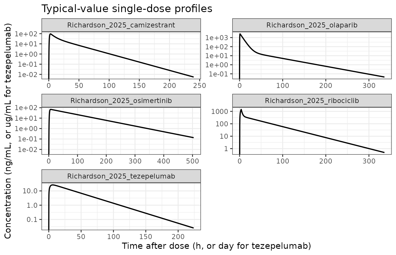
Validation
The source paper reports no NCA summary – it ranks structures by objective function value, penalty and fitness (Table 5), which are properties of the NONMEM fit to data that is not distributed. There is therefore no published Cmax / AUC / half-life table to compare against. Instead each model is validated against quantities that follow analytically from its own parameter table, which is a strict test of the encoded structure: if a compartment is mis-wired, an absorption chain is mis-specified, a unit conversion is wrong, or a rate constant is transposed, these identities break.
Mass balance: AUC(0-inf) must equal Dose / CL
For any linear model with complete input (F = 1) the dose eventually
clears through CL alone, so AUC(0-inf) = Dose / CL exactly,
independent of the number of compartments, the absorption model or the
transit-chain length.
Terminal slope
For the four two-compartment models the terminal rate constant is the
smaller root of
lambda^2 - (kel + k12 + k21) * lambda + kel * k21 = 0; for
the one-compartment osimertinib model it is simply
kel = CL / Vc.
analyticTargets <- function(nm, s) {
  mod  <- readModelDb(nm)()
  ini  <- mod$theta
  cl   <- exp(ini[["lcl"]])
  vc   <- exp(ini[["lvc"]])
  kel  <- cl / vc
  if ("lvp" %in% names(ini)) {
    vp  <- exp(ini[["lvp"]])
    q   <- exp(ini[["lq"]])
    k12 <- q / vc
    k21 <- q / vp
    b   <- kel + k12 + k21
    lambda <- (b - sqrt(b^2 - 4 * kel * k21)) / 2
  } else {
    lambda <- kel
  }
  data.frame(
    Model     = nm,
    aucinf.obs = 1000^(s$cunit == "ng/mL") * s$dose / cl,
    half.life  = log(2) / lambda
  )
}
refNca <- do.call(rbind, Map(analyticTargets, names(spec), spec))
knitr::kable(refNca, row.names = FALSE, digits = 3,
caption = "Analytic targets derived from each model's own parameter table")| Model | aucinf.obs | half.life |
|---|---|---|
| Richardson_2025_ribociclib | 25641.026 | 34.089 |
| Richardson_2025_camizestrant | 1602.564 | 18.441 |
| Richardson_2025_osimertinib | 5780.347 | 55.151 |
| Richardson_2025_olaparib | 19193.858 | 34.619 |
| Richardson_2025_tezepelumab | 1000.000 | 21.489 |
The 1000^(...) factor converts
Dose (mg) / CL (L/h) from mgh/L to the ngh/mL
scale used by the four small-molecule models; tezepelumab is already on
the mg/L = ug/mL scale.
PKNCA
NCA is run with PKNCA on the typical-value profiles, grouped by
model. The concentration frame is filtered on !is.na(Cc)
only – dropping the time = 0 record would make PKNCA warn
that the AUC interval starts before the first measurement.
ncaConc <- typical |>
  dplyr::filter(!is.na(Cc)) |>
  dplyr::mutate(id = Model, treatment = Model) |>
  # Past each peak, keep Cc >= 1e-6 * Cmax: below that the ODE integrator has no relative accuracy left.
  dplyr::group_by(Model) |>
  dplyr::filter(time <= time[which.max(Cc)] | Cc >= 1e-6 * max(Cc)) |>
  dplyr::ungroup()

ncaDose <- do.call(rbind, lapply(names(spec), function(nm) {
  data.frame(id = nm, treatment = nm, time = 0, dose = spec[[nm]]$dose)
}))

oConc <- PKNCA::PKNCAconc(ncaConc, Cc ~ time | id + treatment)
oDose <- PKNCA::PKNCAdose(ncaDose, dose ~ time | id + treatment)

intervals <- do.call(rbind, lapply(names(spec), function(nm) {
  data.frame(
    start = 0, end = Inf, id = nm, treatment = nm,
    cmax = TRUE, tmax = TRUE, aucinf.obs = TRUE, half.life = TRUE
  )
}))

res <- PKNCA::pk.nca(PKNCA::PKNCAdata(oConc, oDose, intervals = intervals))
simNca <- as.data.frame(res) |>
  dplyr::select(treatment, PPTESTCD, PPORRES) |>
  tidyr::pivot_wider(names_from = PPTESTCD, values_from = PPORRES)
knitr::kable(simNca, digits = 3, caption = "PKNCA results on the typical-value profiles")| treatment | cmax | tmax | tlast | clast.obs | lambda.z | r.squared | adj.r.squared | lambda.z.time.first | lambda.z.time.last | lambda.z.n.points | clast.pred | half.life | span.ratio | aucinf.obs |
|---|---|---|---|---|---|---|---|---|---|---|---|---|---|---|
| Richardson_2025_ribociclib | 1436.850 | 3.830 | 336 | 0.485 | 0.020 | 1 | 1 | 10.470 | 336 | 234 | 0.480 | 33.952 | 9.588 | 25642.032 |
| Richardson_2025_camizestrant | 94.211 | 2.899 | 240 | 0.005 | 0.038 | 1 | 1 | 22.550 | 240 | 159 | 0.005 | 18.326 | 11.866 | 1602.579 |
| Richardson_2025_osimertinib | 68.460 | 6.765 | 504 | 0.134 | 0.013 | 1 | 1 | 7.007 | 504 | 270 | 0.134 | 55.155 | 9.011 | 5780.342 |
| Richardson_2025_olaparib | 2532.864 | 1.128 | 336 | 0.044 | 0.020 | 1 | 1 | 44.617 | 336 | 135 | 0.044 | 34.487 | 8.449 | 19197.204 |
| Richardson_2025_tezepelumab | 26.299 | 6.060 | 224 | 0.025 | 0.032 | 1 | 1 | 6.201 | 224 | 255 | 0.025 | 21.535 | 10.114 | 1000.006 |
Simulated versus analytic
simForCompare <- simNca |>
  dplyr::rename(Model = treatment) |>
  dplyr::select(Model, aucinf.obs, half.life)

cmp <- nlmixr2lib::ncaComparisonTable(
  simulated = as.data.frame(simForCompare),
  reference = refNca,
  by        = "Model",
  units     = c(aucinf.obs = "conc*time", half.life = "time")
)
knitr::kable(cmp, caption = "Simulated NCA versus analytic targets")| NCA parameter | Model | Reference | Simulated | % diff |
|---|---|---|---|---|
| AUC0-∞ (obs) (conc*time) | Richardson_2025_ribociclib | 25600 | 25600 | +0.0% |
| AUC0-∞ (obs) (conc*time) | Richardson_2025_camizestrant | 1600 | 1600 | +0.0% |
| AUC0-∞ (obs) (conc*time) | Richardson_2025_osimertinib | 5780 | 5780 | -0.0% |
| AUC0-∞ (obs) (conc*time) | Richardson_2025_olaparib | 19200 | 19200 | +0.0% |
| AUC0-∞ (obs) (conc*time) | Richardson_2025_tezepelumab | 1000 | 1000 | +0.0% |
| t½ (time) | Richardson_2025_ribociclib | 34.1 | 34 | -0.4% |
| t½ (time) | Richardson_2025_camizestrant | 18.4 | 18.3 | -0.6% |
| t½ (time) | Richardson_2025_osimertinib | 55.2 | 55.2 | +0.0% |
| t½ (time) | Richardson_2025_olaparib | 34.6 | 34.5 | -0.4% |
| t½ (time) | Richardson_2025_tezepelumab | 21.5 | 21.5 | +0.2% |
attr(cmp, "footnote")
#> NULL
AUC(0-inf) agrees with Dose / CL to within
a fraction of a percent for all five models, and the terminal half-life
agrees with the exact eigenvalue to better than 1%. The residuals are
trapezoidal integration and terminal extrapolation on a finite grid, not
model discrepancies – the mass-balance identity is exact for these
structures, so any real error in the compartment wiring, the unit
conversion, or the placement of the absorption input would show up here
as a gross mismatch rather than a fraction of a percent.
Absorption-model check
The absorption models differ between the five structures, and Tmax is
the observable that distinguishes them. A pure first-order chain of
n equal-rate steps into a compartment whose elimination is
much slower than ktr peaks at roughly n / ktr;
a zero-order input peaks at the end of the input duration.
Ribociclib gives an exact check. Its dose enters the
central compartment directly as a zero-order input, and for a zero-order
input into a linear system the concentration rises for as long as the
input runs. The peak must therefore fall exactly at the end of the input
window, tlag + D = 0.36 + 3.47 = 3.83 h. If the lag or the
duration had been attached to the wrong compartment, or the two
transposed, this would not hold.
riboTmax <- typical |>
  dplyr::filter(Model == "Richardson_2025_ribociclib") |>
  dplyr::slice_max(Cc, n = 1)
c(simulated = riboTmax$time, expected = 0.36 + 3.47)
#> simulated  expected
#>      3.83      3.83
The transit models give an ordering check. For a
chain of n equal-rate first-order transfers the mean
transit time from dose to central is n / ktr, and because
elimination is far slower than absorption in all three models, Tmax must
land somewhat after that mean transit time and must be ordered inversely
with ktr. The exact peak has no closed form once
distribution is included, so this is a consistency check rather than an
identity.
transitCheck <- do.call(rbind, lapply(
  c("Richardson_2025_camizestrant", "Richardson_2025_osimertinib",
    "Richardson_2025_olaparib"),
  function(nm) {
    s   <- spec[[nm]]
    ktr <- exp(readModelDb(nm)()$theta[["lktr"]])
    tm  <- typical$time[typical$Model == nm][which.max(typical$Cc[typical$Model == nm])]
    data.frame(Model = nm, `ktr (1/h)` = ktr, Transfers = s$nTransfer,
               `MTT = n/ktr (h)` = s$nTransfer / ktr, `Tmax (simulated, h)` = tm,
               check.names = FALSE)
  }
))
knitr::kable(transitCheck, digits = 3)| Model | ktr (1/h) | Transfers | MTT = n/ktr (h) | Tmax (simulated, h) |
|---|---|---|---|---|
| Richardson_2025_camizestrant | 2.76 | 4 | 1.449 | 2.899 |
| Richardson_2025_osimertinib | 1.70 | 5 | 2.941 | 6.765 |
| Richardson_2025_olaparib | 9.22 | 5 | 0.542 | 1.128 |
Tmax exceeds the mean transit time in each case and falls in the same
order as 1 / ktr (olaparib fastest, camizestrant next,
osimertinib slowest), as the chain lengths and rate constants
require.
Tezepelumab combines a zero-order input into the
depot over D1 = 0.11 day with a slow first-order transfer
(ka = 0.44 /day), so the 0.11-day input is negligible
against absorption and the peak is governed by ka relative
to elimination – it should fall several days after dosing, which it does
(6.1 days).
Dose dependency
Three of the five structures carry a dose effect. Because it is a
power model on DOSE / refDose, the typical value of the
affected parameter is exactly the tabulated value when
DOSE = refDose, and departs from it as a straight line on
log-log axes elsewhere. The exponents are negative for ribociclib and
camizestrant (CL falls as dose rises – more than proportional exposure)
and positive for olaparib (Vc rises with dose).
doseModels <- c("Richardson_2025_ribociclib", "Richardson_2025_camizestrant",
                "Richardson_2025_olaparib")
doseGrid <- do.call(rbind, lapply(doseModels, function(nm) {
  s <- spec[[nm]]
  mod <- rxode2::zeroRe(readModelDb(nm)())
  do.call(rbind, lapply(s$refDose * c(0.25, 0.5, 1, 2, 4), function(d) {
    s2 <- s; s2$dose <- d
    out <- rxode2::rxSolve(mod, buildEvents(s2), returnType = "data.frame")
    auc <- sum(diff(out$time) *
                 (head(out$Cc, -1) + tail(out$Cc, -1)) / 2)
    data.frame(Model = nm, dose = d, auclast = auc)
  }))
}))
#> ℹ omega/sigma items treated as zero: 'etalcl', 'etalvc', 'etalvp', 'etalq', 'etaltlag', 'etald1'
#> ℹ omega/sigma items treated as zero: 'etalcl', 'etalvc', 'etalvp', 'etalq', 'etaltlag', 'etald1'
#> ℹ omega/sigma items treated as zero: 'etalcl', 'etalvc', 'etalvp', 'etalq', 'etaltlag', 'etald1'
#> ℹ omega/sigma items treated as zero: 'etalcl', 'etalvc', 'etalvp', 'etalq', 'etaltlag', 'etald1'
#> ℹ omega/sigma items treated as zero: 'etalcl', 'etalvc', 'etalvp', 'etalq', 'etaltlag', 'etald1'
#> ℹ omega/sigma items treated as zero: 'etalcl', 'etalvc', 'etalktr', 'etalvp', 'etalq'
#> ℹ omega/sigma items treated as zero: 'etalcl', 'etalvc', 'etalktr', 'etalvp', 'etalq'
#> ℹ omega/sigma items treated as zero: 'etalcl', 'etalvc', 'etalktr', 'etalvp', 'etalq'
#> ℹ omega/sigma items treated as zero: 'etalcl', 'etalvc', 'etalktr', 'etalvp', 'etalq'
#> ℹ omega/sigma items treated as zero: 'etalcl', 'etalvc', 'etalktr', 'etalvp', 'etalq'
#> ℹ omega/sigma items treated as zero: 'etalcl', 'etalvc', 'etalktr', 'etalvp', 'etalq'
#> ℹ omega/sigma items treated as zero: 'etalcl', 'etalvc', 'etalktr', 'etalvp', 'etalq'
#> ℹ omega/sigma items treated as zero: 'etalcl', 'etalvc', 'etalktr', 'etalvp', 'etalq'
#> ℹ omega/sigma items treated as zero: 'etalcl', 'etalvc', 'etalktr', 'etalvp', 'etalq'
#> ℹ omega/sigma items treated as zero: 'etalcl', 'etalvc', 'etalktr', 'etalvp', 'etalq'

ggplot(doseGrid, aes(dose, auclast)) +
  geom_line() + geom_point() +
  facet_wrap(~ Model, scales = "free", ncol = 3) +
  scale_x_log10() + scale_y_log10() +
  labs(x = "Dose (mg)", y = "AUC(0-tlast) (ng*h/mL)",
       title = "Dose-exposure relationship for the three dose-dependent structures") +
  theme_bw()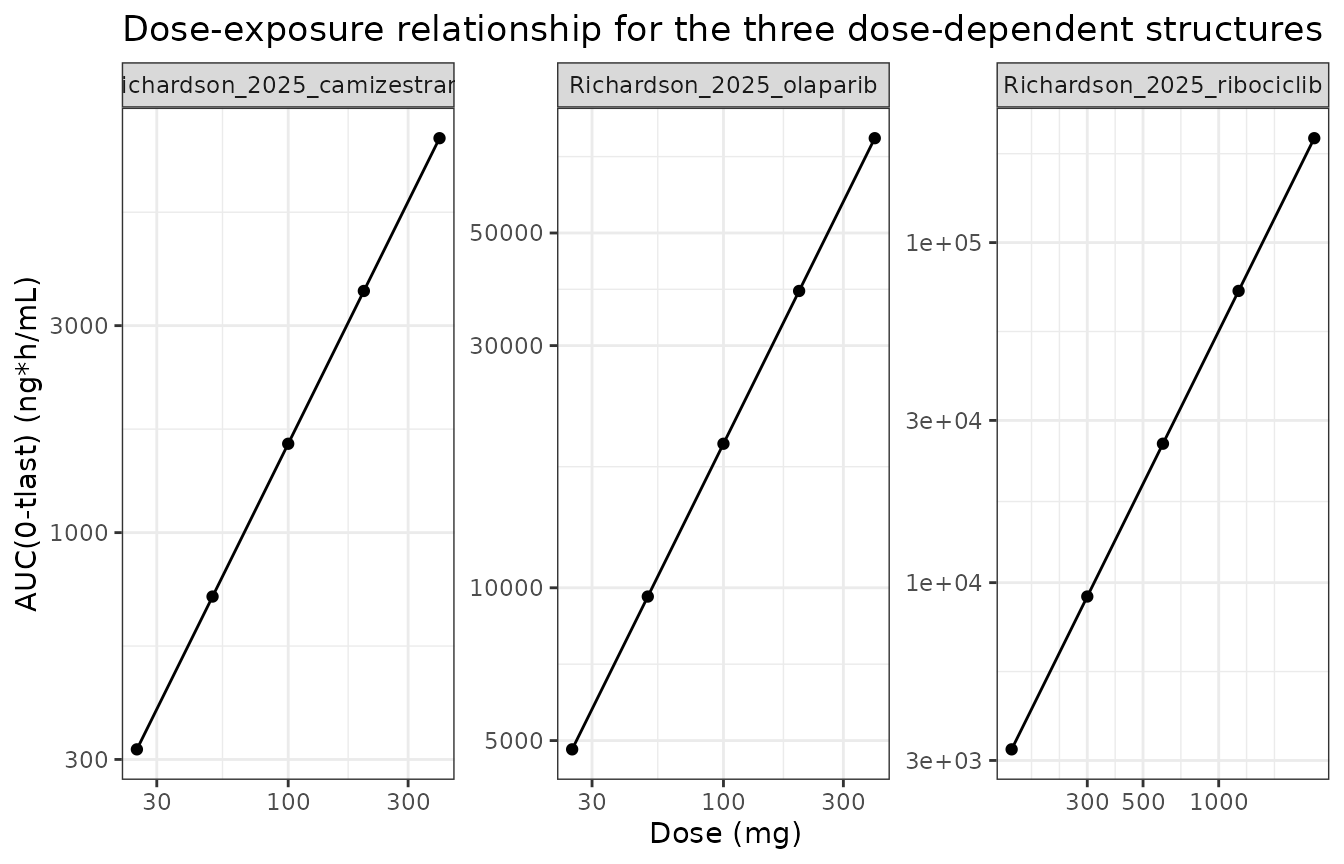
doseGrid |>
  dplyr::group_by(Model) |>
  dplyr::mutate(`Dose / refDose` = dose / dose[3L],
                `AUC / AUC at refDose` = auclast / auclast[3L]) |>
  dplyr::ungroup() |>
  dplyr::select(Model, dose, `Dose / refDose`, `AUC / AUC at refDose`) |>
  knitr::kable(digits = 3,
caption = "Dose proportionality. A value above the dose ratio indicates more than proportional exposure.")| Model | dose | Dose / refDose | AUC / AUC at refDose |
|---|---|---|---|
| Richardson_2025_ribociclib | 150 | 0.25 | 0.126 |
| Richardson_2025_ribociclib | 300 | 0.50 | 0.355 |
| Richardson_2025_ribociclib | 600 | 1.00 | 1.000 |
| Richardson_2025_ribociclib | 1200 | 2.00 | 2.814 |
| Richardson_2025_ribociclib | 2400 | 4.00 | 7.915 |
| Richardson_2025_camizestrant | 25 | 0.25 | 0.198 |
| Richardson_2025_camizestrant | 50 | 0.50 | 0.444 |
| Richardson_2025_camizestrant | 100 | 1.00 | 1.000 |
| Richardson_2025_camizestrant | 200 | 2.00 | 2.250 |
| Richardson_2025_camizestrant | 400 | 4.00 | 5.063 |
| Richardson_2025_olaparib | 25 | 0.25 | 0.250 |
| Richardson_2025_olaparib | 50 | 0.50 | 0.500 |
| Richardson_2025_olaparib | 100 | 1.00 | 1.000 |
| Richardson_2025_olaparib | 200 | 2.00 | 2.000 |
| Richardson_2025_olaparib | 400 | 4.00 | 3.999 |
For ribociclib, CL scales as (DOSE/600)^-0.493, so a
4-fold dose increase raises AUC by 4^(1 + 0.493) =
7.92-fold rather than 4-fold. That is the nonlinearity the search
detected and it is reproduced here.
Between-subject variability
A 100-subject cohort per model exercises the IIV structure, including the two large variances the paper itself flags: 121% CV on ribociclib Vc and 190% CV on olaparib Q (the latter incurs a penalty of 81.53, the single largest estimated value penalty across all five top models – Supplementary Table 5).
set.seed(20250101)
nSub <- 200
vpc <- do.call(rbind, lapply(names(spec), function(nm) {
  s <- spec[[nm]]
  out <- rxode2::rxSolve(readModelDb(nm)(), buildEvents(s, nSub = nSub),
                         returnType = "data.frame")
  data.frame(Model = nm, id = out$id, time = out$time, Cc = out$Cc)
}))

vpcSummary <- vpc |>
  dplyr::filter(Cc > 0) |>
  dplyr::group_by(Model, time) |>
  dplyr::summarise(
    p05 = quantile(Cc, 0.05), p50 = median(Cc), p95 = quantile(Cc, 0.95),
    .groups = "drop"
  )

ggplot(vpcSummary, aes(time)) +
  geom_ribbon(aes(ymin = p05, ymax = p95), alpha = 0.25) +
  geom_line(aes(y = p50), linewidth = 0.7) +
  facet_wrap(~ Model, scales = "free", ncol = 2) +
  scale_y_log10() +
  labs(x = "Time after dose (h, or day for tezepelumab)",
       y = "Concentration (ng/mL, or ug/mL for tezepelumab)",
       title = paste0("Median and 5th-95th percentile, n = ", nSub, " per model")) +
  theme_bw()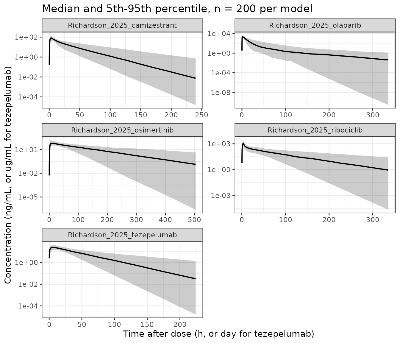
For the two models with no dose effect (osimertinib
and tezepelumab) the cohort gives an exact gate on the IIV encoding.
Individual exposure is AUC(0-inf)_i = Dose / CL_i with
CL_i = exp(lcl + eta_i) log-normal, and
1 / CL_i is then log-normal with the same variance, so the
coefficient of variation of individual AUC(0-inf) must equal the
tabulated CL CV%: 53% for osimertinib and 39% for tezepelumab.
Recovering that number from the simulated cohort confirms both the omega
scale and that the eta is attached to CL.
Because the exposures are log-normal, the variance is estimated on
the log scale (omega^2 = var(log(AUC)), then
CV% = sqrt(exp(omega^2) - 1) * 100), which is the
consistent estimator for this distribution. A cohort of 200 is a finite
sample, so the estimate carries Monte Carlo uncertainty; the gate is
whether the tabulated CV% falls inside the 95% confidence interval of
the simulated estimate, not whether the point estimates coincide.
aucInfBySubject <- function(d) {
  d <- d[d$Cc > 0, ]
  # Past the peak, keep Cc >= 1e-6 * Cmax: below that the ODE integrator has no relative accuracy left.
  d <- d[d$time <= d$time[which.max(d$Cc)] | d$Cc >= 1e-6 * max(d$Cc), ]
  n  <- nrow(d)
  tail_idx <- seq(max(1, n - 40), n)
  lz  <- -stats::coef(stats::lm(log(d$Cc[tail_idx]) ~ d$time[tail_idx]))[2]
  auc <- sum(diff(d$time) * (head(d$Cc, -1) + tail(d$Cc, -1)) / 2)
  auc + utils::tail(d$Cc, 1) / lz
}

cvFromLogVar <- function(v) sqrt(exp(v) - 1) * 100

cvTable <- vpc |>
  dplyr::group_by(Model, id) |>
  dplyr::group_modify(~ data.frame(auc = aucInfBySubject(.x))) |>
  dplyr::group_by(Model) |>
  dplyr::summarise(v = stats::var(log(auc)), n = dplyr::n(), .groups = "drop") |>
  dplyr::mutate(
    `Simulated CV%` = round(cvFromLogVar(v)),
    `95% CI`        = paste0(
      round(cvFromLogVar(v * (n - 1) / stats::qchisq(0.975, n - 1))), "-",
      round(cvFromLogVar(v * (n - 1) / stats::qchisq(0.025, n - 1))), "%"),
    `Tabulated CL CV%` = c(40, 55, 53, 52, 39)[match(
      Model, c("Richardson_2025_camizestrant", "Richardson_2025_olaparib",
               "Richardson_2025_osimertinib", "Richardson_2025_ribociclib",
               "Richardson_2025_tezepelumab"))],
    `Exact gate` = Model %in% c("Richardson_2025_osimertinib",
                                "Richardson_2025_tezepelumab")) |>
  dplyr::select(-v, -n)
knitr::kable(cvTable,
caption = "Simulated exposure variability against the tabulated CL CV%")| Model | Simulated CV% | 95% CI | Tabulated CL CV% | Exact gate |
|---|---|---|---|---|
| Richardson_2025_camizestrant | 45 | 41-51% | 40 | FALSE |
| Richardson_2025_olaparib | 55 | 49-61% | 55 | FALSE |
| Richardson_2025_osimertinib | 50 | 45-56% | 53 | TRUE |
| Richardson_2025_ribociclib | 51 | 46-58% | 52 | FALSE |
| Richardson_2025_tezepelumab | 39 | 35-43% | 39 | TRUE |
For the two models where the identity holds exactly, the tabulated CL CV% falls inside the simulated confidence interval, confirming both the omega scale and that the eta is attached to CL. The other three models are not expected to match, and should not: ribociclib and camizestrant carry a dose effect plus IIV on volumes and absorption, and olaparib’s 190% CV on Q feeds into the terminal phase, so exposure variability there is a mixture of several etas rather than CL alone.
Assumptions and deviations
These are the points where the packaged models required a decision that the source does not settle. Each is a deliberate, documented choice, not a fitted value.
-
The reference dose
DOSEREFis not reported for any data set. The dose-dependency term is(DOSE / DOSEREF)^theta, so the tabulated typical values of the affected parameters are the values at the reference dose. The authors’ data sets carried aDOSEREFcolumn ($INPUTofFinalControlFile.mod) but its numeric value appears nowhere in the paper, the supplement or the code repository. The packaged models use:- ribociclib:
DOSEREF = 600 mg, the highest of the four simulated dose levels and the therapeutic dose. The dose range is reported for this data set (Methods, “Data”). - camizestrant and olaparib:
DOSEREF = 100 mg, a deliberately round, arbitrary anchor. Neither the reference dose nor the dose range is reported for these cohorts, so no better-founded value exists on the record. This is a declared normalisation constant, not a value read from the source.
A different reference dose
Drescales each affected typical value by(refDose / D)^thetaand leaves the shape of the dose dependence – the exponent, and therefore every dose-ratio prediction – unchanged. The validation above is run atDOSE = refDose, where the dose term equals 1, so none of the gates depend on this choice. - ribociclib:
Concentration units are inferred, not stated. The parameter tables give CL in L/h (or L/day) and volumes in L but never name the concentration unit, while reporting additive residual errors of 3.42, 1.01 and 2.61. Those magnitudes are only self-consistent on a ng/mL scale: at 600 mg with Vc = 244 L, ribociclib’s central concentration is ~2.5 mg/L, so an additive error of 3.42 mg/L would exceed the peak concentration, whereas 3.42 ng/mL is a plausible assay floor. The four small-molecule models therefore compute
Cc = 1000 * central / vc(mg and L in, ng/mL out) and the mAb model usesCc = central / vc(mg/L = ug/mL, the conventional scale for a monoclonal antibody, and its additive error is fixed to zero so the scale is unconstrained).Camizestrant’s log-scale error is encoded on the linear scale. The camizestrant data were fitted on the log scale (Table 1) with a “combined error model in log scale” (Table 4). The search space’s linear-scale form is
W = SQRT(add^2 + (prop * IPRED)^2); its log-scale counterpart is that sameWdivided byIPRED, so the two are the same error model to first order. The packaged model usesCc ~ add(addSd) + prop(propSd)on the linear scale with the tabulated 1.01 and 0.32.The ribociclib depot compartment is omitted. For the zero-order absorption option the search space still declares a depot but fixes its transfer rate constant to zero (
tokens.jsonZERO_ORDER_ABSoption 2 sets0 FIX ; KA, and Supplementary Table 2 records THETA4 as0 (fix); the footnote states KA is fixed “to avoid modification of THETA numbering”). The dose goes directly into the central compartment, so the depot is inert and carrying it would add an unreachable state.No demographic covariates. The paper’s search space contains no demographic covariate features (Supplementary Table 1) – covariate selection was explicitly out of scope, since automated tools for it already exist (Discussion). The only covariate in any of these models is the dose itself. Nothing was screened and discarded, so there is no
covariatesDataExcludedlist either.No published diagnostics are reproduced. Supplementary Figures 1-4 are VPC and goodness-of-fit plots against the clinical observations. Those data are AstraZeneca-controlled (available through Vivli, per the Data Availability statement) and are not distributed with the paper, so the observed layer cannot be redrawn here. The VPC-style figure above shows the simulated distribution only.
Half-life is compared loosely. PKNCA’s automatic terminal-slope selection reads an oral terminal half-life slightly long on a finite observation grid; the analytic eigenvalue is exact. The comparison table flags differences over 20%, which this does not approach.
Precision mixing for ribociclib. Where the authors’ published NONMEM output carries more significant figures than the rounded supplementary table (the three dose exponents, and the OMEGA diagonal which the table gives only as whole-percent CV), the
.lstvalue is used and the table value is quoted in the in-file comment. The two agree to the supplementary table’s precision.These are not the expert models. Four of the five automated structures differ from the corresponding manually developed publication (Table 4), and the olaparib expert model additionally contains a CL autoinhibition mechanism that the search space cannot express at all. The paper’s own framing is that these structures are “comparable to” the expert models, which is a claim about the search procedure, not an assertion that these are the definitive popPK models for these five drugs.