Osimertinib and AZ5104 (Yang 2025)
Source:vignettes/articles/Yang_2025_osimertinib.Rmd
Yang_2025_osimertinib.RmdModel
Yang_2025_osimertinib is the FLAURA2 update of the
osimertinib parent-metabolite population PK model. Yang 2025 pooled
52,338 plasma samples from 2,196 patients with EGFR-mutated advanced
NSCLC across six studies (AURA and its extension, AURA2, AURA3, FLAURA,
ADAURA and FLAURA2) and re-estimated the structure first published by
Brown 2017: first-order oral absorption into a one-compartment parent
disposition, feeding a one-compartment metabolite (AZ5104) in series,
with first-order elimination from both.
The analysis exists to answer one question – does adding pemetrexed plus platinum chemotherapy change osimertinib PK? – and its answer is no. “Addition of chemotherapy” was tested by forward inclusion on both parent and metabolite clearance and was not significant on either (Table S2), so it does not appear in the model at all. The covariates that were retained (weight, albumin, race) were all judged to have no clinically meaningful effect on exposure.
mod <- nlmixr2lib::readModelDb("Yang_2025_osimertinib")
mod
#> function() {
#>   description <- paste(
#>     "Joint parent-metabolite population PK model for osimertinib and its",
#>     "active metabolite AZ5104 in 2,196 patients with EGFR-mutated advanced",
#>     "non-small cell lung cancer (NSCLC), pooled across six studies (AURA,",
#>     "AURA2, AURA3, FLAURA, ADAURA, and FLAURA2) (Yang 2025). This is the",
#>     "FLAURA2 update of the earlier Brown 2017 model: it retains the same",
#>     "published structure (first-order oral absorption into a one-compartment",
#>     "parent disposition, feeding a one-compartment metabolite in series, with",
#>     "first-order elimination from both) and re-estimates it on the pooled",
#>     "dataset that adds the FLAURA2 osimertinib-plus-chemotherapy arm. The",
#>     "fraction of parent clearance appearing as AZ5104 is fixed at 0.25.",
#>     "Retained covariates are baseline body weight and baseline serum albumin",
#>     "on parent CL/F and V/F, baseline body weight, baseline serum albumin and",
#>     "race (Japanese and Asian-other, each vs a White reference) on AZ5104",
#>     "CL/F, and baseline serum albumin on AZ5104 V/F. Chinese and Other race",
#>     "indicators were carried in the final control stream but their",
#>     "coefficients were fixed to zero after backward elimination found them",
#>     "non-significant. Adding chemotherapy was tested on both parent and",
#>     "metabolite clearance and was not significant, i.e. the model found no",
#>     "pemetrexed-platinum drug interaction. No covariate had a clinically",
#>     "meaningful effect. Concentrations are in nM, matching the source.",
#>     sep = " "
#>   )
#>   reference <- paste(
#>     "Yang J, Olabode D, Sawant-Basak A, Baldry R, Vishwanathan K, Bachina S,",
#>     "Todd A, Ghiorghiu D, Rukazenkov Y, Zhou D, Shahraz A. Population",
#>     "Pharmacokinetics and Exposure-Response Analysis of First-Line",
#>     "Osimertinib Plus Chemotherapy in Patients with EGFR-Mutated Advanced",
#>     "NSCLC. Clin Pharmacol Ther. 2025;118(5):1110-1120.",
#>     "doi:10.1002/cpt.3759",
#>     sep = " "
#>   )
#>   vignette <- "Yang_2025_osimertinib"
#>   units <- list(time = "h", dosing = "mg", concentration = "nM")
#>
#>   # Issue #482: what each ODE state holds, in what amount units, in what
#>   # biological matrix. Amounts are carried in mg of parent-mass equivalent
#>   # throughout, exactly as in the source NONMEM control stream: the
#>   # central -> metabolite transfer is 1:1 in amount (no molar
#>   # stoichiometric correction), and each analyte's concentration is then
#>   # formed with its OWN molecular weight via the control stream's scaling
#>   # factors S2 = V1 * 499.61 / 1e6 and S3 = VM1 * 485.59 / 1e6. Verified
#>   # against Table S5: this convention reproduces the observed AZ5104
#>   # steady-state AUC to within 1%, whereas a molar 1:1 transfer is low by
#>   # about 3%.
#>   compartmentData <- list(
#>     depot = list(analyte = "osimertinib", units = "mg", specimen = "administration site", verified = TRUE),
#>     central = list(analyte = "osimertinib", units = "mg", specimen = "plasma", verified = TRUE),
#>     central_az5104 = list(
#>       analyte = "AZ5104",
#>       units = "mg (parent-mass equivalent)",
#>       specimen = "plasma",
#>       verified = TRUE
#>     )
#>   )
#>
#>   covariateData <- list(
#>     WT = list(
#>       description = "Total body weight at baseline.",
#>       units = "kg",
#>       type = "continuous",
#>       reference_value = "62 kg (Yang 2025 Table 1 overall median; the reference used in Eqs 2-4 and in the Figure 3 forest-plot reference patient).",
#>       notes = "Power (allometric-form) effect on parent CL/F (exponent 0.36), parent V/F (0.64) and AZ5104 CL/F (0.74). The source control stream maps a missing weight (coded -999) onto a covariate factor of 1, i.e. the typical value; this implementation has no missingness code and expects an observed weight.",
#>       source_name = "WT (Yang 2025 supplementary NONMEM control stream $INPUT)"
#>     ),
#>     ALB = list(
#>       description = "Serum albumin at baseline.",
#>       units = "g/L",
#>       type = "continuous",
#>       reference_value = "40 g/L (Yang 2025 Table 1 overall median; the reference used in Eqs 2-5).",
#>       notes = "Power effect on parent CL/F (exponent 0.67), parent V/F (1.57), AZ5104 CL/F (0.72) and AZ5104 V/F (-0.65). The AZ5104 V/F exponent is NEGATIVE: Table 2 prints its magnitude (0.65) only, but Eq 5 and $THETA(13) = -0.652465 both carry the sign. Reported in g/L (SI); US-convention g/dL values must be multiplied by 10.",
#>       source_name = "BALB (Yang 2025 supplementary NONMEM control stream $INPUT)"
#>     ),
#>     RACE_ASIAN_OTH = list(
#>       description = "Asian-other race indicator (1 = Asian heritage other than Chinese or Japanese, 0 = otherwise).",
#>       units = "(binary)",
#>       type = "binary",
#>       reference_category = "0 (the paper-defined race reference category is White).",
#>       notes = "Linear additive effect (1 + 0.161274 * RACE_ASIAN_OTH) on AZ5104 CL/F, i.e. 16.1% higher metabolite clearance than a White patient. Corresponds to ETHL = 1 in the source control stream. Yang 2025 carries White (reference), Asian-other, Chinese, Japanese and Other as five mutually exclusive levels; the dominant reference cohort is White, not Chinese.",
#>       source_name = "ETHL = 1 (Yang 2025 supplementary NONMEM control stream); 'Asian (excluding Chinese and Japanese)' (Table 1); 'Asian (NonCHN or nonJPN) on CLm/F' (Table 2)"
#>     ),
#>     RACE_JAPANESE = list(
#>       description = "Japanese-heritage race indicator (1 = Japanese, 0 = otherwise).",
#>       units = "(binary)",
#>       type = "binary",
#>       reference_category = "0 (the paper-defined race reference category is White).",
#>       notes = "Linear additive effect (1 + 0.181966 * RACE_JAPANESE) on AZ5104 CL/F, i.e. 18.2% higher metabolite clearance than a White patient. Corresponds to ETHL = 3 in the source control stream.",
#>       source_name = "ETHL = 3 (Yang 2025 supplementary NONMEM control stream); 'JPN on CLm/F' (Table 2)"
#>     ),
#>     RACE_CHINESE = list(
#>       description = "Chinese-heritage race indicator (1 = Chinese, 0 = otherwise).",
#>       units = "(binary)",
#>       type = "binary",
#>       reference_category = "0 (the paper-defined race reference category is White).",
#>       notes = "Carried in the final model structure but with its coefficient FIXED TO ZERO, so it has no effect on AZ5104 CL/F. Backward elimination (Table S2) found that removing Chinese from CLm/F was 'Not significant', and the source control stream accordingly holds $THETA(15) at '0 FIX' for ETHL = 2. Retained here so the covariate screen is auditable rather than silently dropped.",
#>       source_name = "ETHL = 2 (Yang 2025 supplementary NONMEM control stream $THETA(15), 0 FIX)"
#>     ),
#>     RACE_OTHER = list(
#>       description = "Race-category 'Other' indicator (1 = Hispanic/Latino, Native American, Native Alaskan/Inuit, Native Hawaiian/Pacific Islander, African, African-American, African-Caribbean, or missing; 0 = otherwise).",
#>       units = "(binary)",
#>       type = "binary",
#>       reference_category = "0 (the paper-defined race reference category is White).",
#>       notes = "Carried in the final model structure but with its coefficient FIXED TO ZERO, so it has no effect on AZ5104 CL/F. Backward elimination (Table S2) found that removing other ethnicity from CLm/F was 'Not significant', and the source control stream accordingly holds $THETA(17) at '0 FIX' for ETHL = 99. The composite membership is defined in the Yang 2025 Table 1 footnote a.",
#>       source_name = "ETHL = 99 (Yang 2025 supplementary NONMEM control stream $THETA(17), 0 FIX)"
#>     )
#>   )
#>
#>   # Covariates that Yang 2025 evaluated but did not retain. Recorded so the
#>   # covariate screen stays auditable; none is referenced in model().
#>   covariatesDataExcluded <- list(
#>     AGE = list(
#>       description = "Age at baseline.",
#>       units = "years",
#>       type = "continuous",
#>       notes = "Median 62.0 (range 25.0-91.0) overall (Table 1). Not retained in the final PopPK model."
#>     ),
#>     CRCL = list(
#>       description = "Creatinine clearance at baseline.",
#>       units = "mL/min",
#>       type = "continuous",
#>       notes = "Forward inclusion on parent CL/F was 'Not significant' (Table S2)."
#>     ),
#>     RENAL_IMPAIRMENT = list(
#>       description = "Grouped renal impairment status (normal / mild / moderate-severe).",
#>       units = "(category)",
#>       type = "categorical",
#>       notes = "Forward inclusion on parent CL/F and AZ5104 CL/F was 'Not significant' (Table S2); the paper concludes no renal dose adjustment is needed."
#>     ),
#>     HEPATIC_IMPAIRMENT = list(
#>       description = "Grouped hepatic impairment status (normal / at least mild).",
#>       units = "(category)",
#>       type = "categorical",
#>       notes = "Forward inclusion on parent CL/F and AZ5104 CL/F was 'Not significant' (Table S2); the paper concludes no hepatic dose adjustment is needed."
#>     ),
#>     CHEMO_COMBINATION = list(
#>       description = "Co-administration of pemetrexed plus platinum chemotherapy.",
#>       units = "(binary)",
#>       type = "binary",
#>       notes = "The pre-specified covariate of interest for this analysis. Forward inclusion on both parent CL/F and AZ5104 CL/F was 'Not significant' (Table S2), i.e. no osimertinib-chemotherapy drug interaction; this is the paper's central PK finding."
#>     )
#>   )
#>
#>   population <- list(
#>     species = "human",
#>     n_subjects = 2196,
#>     n_studies = 6,
#>     n_samples = 52338,
#>     studies = "AURA (including its extension phase), AURA2, AURA3, FLAURA, ADAURA, FLAURA2 (NCT04035486)",
#>     disease_state = "EGFR-mutated locally advanced or metastatic non-small cell lung cancer (NSCLC)",
#>     age_range = "25.0-91.0 years (overall median 62.0; mean 61.5, SD 10.7)",
#>     weight_range = "29.0-128 kg (overall median 62.0; mean 63.5, SD 14.1)",
#>     albumin_range = "17.0-53.3 g/L (overall median 40.0; mean 39.7, SD 4.92)",
#>     crcl_range = "20.5-196 mL/min (overall median 82.1; mean 85.1, SD 26.8)",
#>     bmi_range = "12.9-42.6 kg/m2 (overall median 23.4)",
#>     sex_female_pct = 64.5,
#>     race_ethnicity = list(
#>       White = 26.6,
#>       `Asian (excluding Chinese and Japanese)` = 22.9,
#>       Chinese = 22.8,
#>       Japanese = 17.5,
#>       Other = 10.2
#>     ),
#>     line_of_therapy = list(`First-line` = 38.5, `Second-line` = 21.3, `Third-line and later` = 25.4, Adjuvant = 14.8),
#>     who_ps = list(`0` = 40.8, `1` = 59.2),
#>     dose_range = "Osimertinib 80 mg once daily (reduction to 40 mg once daily permitted for toxicity). In the FLAURA2 combination arm, given with pemetrexed 500 mg/m2 plus either cisplatin 75 mg/m2 or carboplatin AUC 5 mg/mL/min on Day 1 of 21-day cycles for 4 cycles, then pemetrexed 500 mg/m2 maintenance every 3 weeks.",
#>     notes = "Demographics reproduced from Yang 2025 Table 1 (Overall, N = 2,196). Of 52,338 plasma samples, 3,636 (7.0%) were removed and 3,250 (6.2%) below-quantification-limit samples were handled by the M1 method. Race percentages are of the overall pooled population; the reference (typical) patient used for the Figure 3 forest plot is a White patient of 62 kg with albumin 40 g/L."
#>   )
#>
#>   ini({
#>     # ---- Structural parameters -------------------------------------------
#>     # Typical values for the reference patient: White, 62 kg, albumin 40 g/L.
#>     # Final estimates are taken at full precision from the $THETA block of the
#>     # supplementary NONMEM control stream ($PROBLEM FINAL MODEL); each rounds
#>     # to the value printed in Table 2 and in Eqs 1-5.
#>     lka           <- log(0.260946);  label("First-order oral absorption rate constant, Ka (1/h)")                       # Yang 2025 $THETA(3) = 0.260946; Table 2 Ka = 0.26; Eq 1
#>     lcl           <- log(14.3452);   label("Apparent total parent clearance, CLptot/F, reference patient (L/h)")        # Yang 2025 $THETA(1) = 14.3452; Table 2 CLptot/F = 14.35; Eq 2
#>     lvc           <- log(1151.11);   label("Apparent parent volume of distribution, Vp/F, reference patient (L)")       # Yang 2025 $THETA(4) = 1151.11; Table 2 Vp/F = 1,151; Eq 3
#>     lcl_az5104    <- log(32.0484);   label("Apparent AZ5104 clearance, CLm/F, reference patient (L/h)")                 # Yang 2025 $THETA(2) = 32.0484; Table 2 CLm/F = 32.05; Eq 4
#>     lvc_az5104    <- log(151.014);   label("Apparent AZ5104 volume of distribution, Vm/F, reference patient (L)")       # Yang 2025 $THETA(6) = 151.014; Table 2 Vm/F = 151; Eq 5
#>
#>     # Fraction of parent clearance appearing as AZ5104. Fixed, not estimated:
#>     # fm, Vm/F and CLm/F are mutually confounded in a joint parent-metabolite
#>     # model fitted to plasma data alone.
#>     fm            <- fixed(0.25);    label("Fraction of parent clearance forming AZ5104 (unitless)")                    # Yang 2025 $THETA(5) = 0.25 FIX; Table 2 Fm = 0.25 (Fixed); Methods "Fm was fixed at 25%"
#>
#>     # ---- Continuous-covariate power effects ------------------------------
#>     # Form: (WT / 62)^exponent and (ALB / 40)^exponent, per Eqs 2-5.
#>     e_wt_cl            <- 0.359774;  label("Power exponent for body weight on parent CL/F (unitless)")                  # Yang 2025 $THETA(7) = 0.359774; Table 2 WT on CLptot/F = 0.36; Eq 2
#>     e_alb_cl           <- 0.674479;  label("Power exponent for albumin on parent CL/F (unitless)")                      # Yang 2025 $THETA(8) = 0.674479; Table 2 ALB on CLptot/F = 0.67; Eq 2
#>     e_wt_vc            <- 0.640227;  label("Power exponent for body weight on parent V/F (unitless)")                   # Yang 2025 $THETA(9) = 0.640227; Table 2 WT on Vp/F = 0.64; Eq 3
#>     e_alb_vc           <- 1.56611;   label("Power exponent for albumin on parent V/F (unitless)")                       # Yang 2025 $THETA(10) = 1.56611; Table 2 ALB on Vp/F = 1.57; Eq 3
#>     e_wt_cl_az5104     <- 0.740376;  label("Power exponent for body weight on AZ5104 CL/F (unitless)")                  # Yang 2025 $THETA(11) = 0.740376; Table 2 WT on CLm/F = 0.74; Eq 4
#>     e_alb_cl_az5104    <- 0.722460;  label("Power exponent for albumin on AZ5104 CL/F (unitless)")                      # Yang 2025 $THETA(12) = 0.722460; Table 2 ALB on CLm/F = 0.72; Eq 4
#>     # NEGATIVE exponent: Table 2 prints only the magnitude (0.65), but Eq 5
#>     # writes (ALB/40)^-0.65 and $THETA(13) = -0.652465 carries the sign.
#>     e_alb_vc_az5104    <- -0.652465; label("Power exponent for albumin on AZ5104 V/F (unitless)")                       # Yang 2025 $THETA(13) = -0.652465; Eq 5 exponent -0.65; Table 2 ALB on Vm/F prints 0.65 unsigned
#>
#>     # ---- Categorical-covariate linear effects ----------------------------
#>     # Form: (1 + coefficient * indicator) on AZ5104 CL/F, per Eq 4 and the
#>     # control stream's CLM1ETHL block. White (ETHL = 0) is the reference.
#>     e_race_asian_oth_cl_az5104 <- 0.161274;  label("Linear coefficient for Asian-other vs White on AZ5104 CL/F (unitless)")  # Yang 2025 $THETA(14) = 0.161274; Table 2 = 0.16; Eq 4 factor 1.16
#>     e_race_japanese_cl_az5104  <- 0.181966;  label("Linear coefficient for Japanese vs White on AZ5104 CL/F (unitless)")     # Yang 2025 $THETA(16) = 0.181966; Table 2 = 0.18; Eq 4 factor 1.18
#>     # Fixed to zero after backward elimination judged them non-significant
#>     # (Table S2); kept so the covariate screen stays visible.
#>     e_race_chinese_cl_az5104   <- fixed(0);  label("Linear coefficient for Chinese vs White on AZ5104 CL/F (unitless; no retained effect)")  # Yang 2025 $THETA(15) = 0 FIX; Table S2 "Removing Chinese from CLm/F: Not significant"
#>     e_race_other_cl_az5104     <- fixed(0);  label("Linear coefficient for Other vs White on AZ5104 CL/F (unitless; no retained effect)")    # Yang 2025 $THETA(17) = 0 FIX; Table S2 "Removing other ethnicity from CLm/F: Not significant"
#>
#>     # ---- Between-subject variability -------------------------------------
#>     # Table 2's "Between subject variability" column is on the VARIANCE scale.
#>     # Confirmed three ways: (i) the values equal the control stream's $OMEGA
#>     # entries exactly; (ii) back-transforming each as a variance via
#>     # sqrt(exp(omega2) - 1) reproduces every published %CV to within 1
#>     # percentage point (46/52/101/85/82% for CLptot/F, CLm/F, Ka, Vp/F, Vm/F),
#>     # whereas reading them as SDs gives 19/24/80/58/55%; (iii) the off-diagonal
#>     # is a $OMEGA BLOCK(2) covariance, not a correlation coefficient -- it
#>     # implies a CLptot/F ~ CLm/F correlation of 0.88, which Table 2's
#>     # "Correlation" row reports unconverted.
#>     etalcl + etalcl_az5104 ~ c(0.191276,
#>                                0.186815, 0.237930)                                # Yang 2025 $OMEGA BLOCK(2); Table 2 IIV on CLptot/F = 0.19, Correlation = 0.19, IIV on CLm/F = 0.24
#>     etalka        ~ 0.699828                                                      # Yang 2025 $OMEGA 3; Table 2 IIV on Ka = 0.70 (%CV 101)
#>     etalvc        ~ 0.542208                                                      # Yang 2025 $OMEGA 4; Table 2 IIV on Vp/F = 0.54 (%CV 85)
#>     etalvc_az5104 ~ 0.512184                                                      # Yang 2025 $OMEGA 5; Table 2 IIV on Vm/F = 0.51 (%CV 82)
#>
#>     # ---- Residual unexplained variability ---------------------------------
#>     # Combined additive plus proportional, estimated separately per analyte.
#>     # The control stream's $ERROR builds W = sqrt(THETA_add^2 + (THETA_prop *
#>     # IPRED)^2) with $SIGMA 1 FIX, so each THETA is a standard deviation on the
#>     # nM concentration scale and maps directly onto add()/prop().
#>     propSd         <- 0.219108;  label("Proportional residual error on osimertinib (fraction)")   # Yang 2025 $THETA(19) = 0.219108; Table 2 parent proportional component = 0.22
#>     addSd          <- 29.5202;   label("Additive residual error on osimertinib (nM)")             # Yang 2025 $THETA(18) = 29.5202; Table 2 parent additive component = 29.52 nM
#>     propSd_az5104  <- 0.231740;  label("Proportional residual error on AZ5104 (fraction)")        # Yang 2025 $THETA(21) = 0.231740; Table 2 metabolite proportional component = 0.23
#>     addSd_az5104   <- 0.358422;  label("Additive residual error on AZ5104 (nM)")                  # Yang 2025 $THETA(20) = 0.358422; Table 2 metabolite additive component = 0.36 nM
#>   })
#>
#>   model({
#>     # Molecular weights used by the source control stream's scaling factors
#>     # S2 = V1 * 499.61 / 1e6 (osimertinib) and S3 = VM1 * 485.59 / 1e6
#>     # (AZ5104, N-desmethyl osimertinib). They convert an amount in mg and a
#>     # volume in L into a concentration in nM, which is the scale on which
#>     # Yang 2025 reports every concentration, the assay range (16-8,010 nM
#>     # osimertinib; 1.65-824 nM AZ5104), the additive residual errors and the
#>     # AUCss quartiles.
#>     mw_parent <- 499.61
#>     mw_az5104 <- 485.59
#>
#>     # Reference covariate values (Yang 2025 Table 1 overall medians; the
#>     # denominators written into Eqs 2-5 and the control stream).
#>     ref_wt  <- 62
#>     ref_alb <- 40
#>
#>     # ---- Individual parameters (Eqs 1-5) ---------------------------------
#>     ka <- exp(lka + etalka)
#>
#>     cl <- exp(lcl + etalcl) *
#>       (WT / ref_wt)^e_wt_cl *
#>       (ALB / ref_alb)^e_alb_cl
#>
#>     vc <- exp(lvc + etalvc) *
#>       (WT / ref_wt)^e_wt_vc *
#>       (ALB / ref_alb)^e_alb_vc
#>
#>     cl_az5104 <- exp(lcl_az5104 + etalcl_az5104) *
#>       (WT / ref_wt)^e_wt_cl_az5104 *
#>       (ALB / ref_alb)^e_alb_cl_az5104 *
#>       (1 + e_race_asian_oth_cl_az5104 * RACE_ASIAN_OTH) *
#>       (1 + e_race_japanese_cl_az5104  * RACE_JAPANESE) *
#>       (1 + e_race_chinese_cl_az5104   * RACE_CHINESE) *
#>       (1 + e_race_other_cl_az5104     * RACE_OTHER)
#>
#>     vc_az5104 <- exp(lvc_az5104 + etalvc_az5104) *
#>       (ALB / ref_alb)^e_alb_vc_az5104
#>
#>     # ---- ODE system ------------------------------------------------------
#>     # Reproduces the control stream's ADVAN7 rate constants exactly:
#>     #   K12 = KA, K20 = CL * (1 - FM) / V1, K23 = CL * FM / V1,
#>     #   K30 = CLM1 / VM1.
#>     # Total efflux from central is therefore cl/vc (the K20 + K23 sum), of
#>     # which the fraction fm is routed to the metabolite. The transfer is 1:1
#>     # in amount with NO molar stoichiometric correction -- that is what the
#>     # source fitted, and it is what reproduces the published AZ5104 exposure
#>     # (see compartmentData above).
#>     d/dt(depot)          <- -ka * depot
#>     d/dt(central)        <-  ka * depot - (cl / vc) * central
#>     d/dt(central_az5104) <-  fm * (cl / vc) * central -
#>       (cl_az5104 / vc_az5104) * central_az5104
#>
#>     # ---- Observations (nM) -----------------------------------------------
#>     Cc        <- central        / (vc        * mw_parent / 1e6)
#>     Cc_az5104 <- central_az5104 / (vc_az5104 * mw_az5104 / 1e6)
#>
#>     Cc        ~ prop(propSd)        + add(addSd)
#>     Cc_az5104 ~ prop(propSd_az5104) + add(addSd_az5104)
#>   })
#> }
#> <environment: 0x55bd52bda1d8>
Population
Yang 2025 Table 1, overall pooled column (N = 2,196):
| Characteristic | Value |
|---|---|
| Age (years) | median 62.0 (range 25.0-91.0); mean 61.5, SD 10.7 |
| Weight (kg) | median 62.0 (range 29.0-128); mean 63.5, SD 14.1 |
| Body mass index (kg/m2) | median 23.4 (range 12.9-42.6) |
| Creatinine clearance (mL/min) | median 82.1 (range 20.5-196) |
| Serum albumin (g/L) | median 40.0 (range 17.0-53.3); mean 39.7, SD 4.92 |
| Sex | 1,416 female (64.5%), 780 male (35.5%) |
| Race | White 584 (26.6%), Asian excluding Chinese and Japanese 502 (22.9%), Chinese 501 (22.8%), Japanese 384 (17.5%), Other 225 (10.2%) |
| WHO performance status | 0: 896 (40.8%); 1: 1,300 (59.2%) |
| Line of therapy | first 38.5%, second 21.3%, third or later 25.4%, adjuvant 14.8% |
Dosing is osimertinib 80 mg once daily, with a permitted reduction to 40 mg once daily for toxicity. In the FLAURA2 combination arm this was given with pemetrexed 500 mg/m2 plus either cisplatin 75 mg/m2 or carboplatin AUC 5 mg/mL/min on Day 1 of 21-day cycles for four cycles, then pemetrexed maintenance every three weeks.
The reference (“typical”) patient used throughout Yang 2025, and used for every typical-value check below, is a White patient of 62 kg with serum albumin 40 g/L – the Table 1 medians and the denominators written into Eqs 2-5.
Source trace
Every value in ini() and every equation in
model(), with its location in the source. The supplementary
NONMEM control stream ($PROBLEM FINAL MODEL) carries the
same values at full precision as the rounded Table 2 entries, so it is
the quoted source where the extra digits matter.
| Model element | Value | Source |
|---|---|---|
lka |
0.260946 1/h | Table 2 (0.26); Eq 1; $THETA(3)
|
lcl (CLptot/F) |
14.3452 L/h | Table 2 (14.35); Eq 2; $THETA(1)
|
lvc (Vp/F) |
1151.11 L | Table 2 (1,151); Eq 3; $THETA(4)
|
lcl_az5104 (CLm/F) |
32.0484 L/h | Table 2 (32.05); Eq 4; $THETA(2)
|
lvc_az5104 (Vm/F) |
151.014 L | Table 2 (151); Eq 5; $THETA(6)
|
fm |
0.25, fixed | Table 2 “0.25 (Fixed)”; Methods;
$THETA(5) 0.25 FIX
|
e_wt_cl |
0.359774 | Table 2 (0.36); Eq 2; $THETA(7)
|
e_alb_cl |
0.674479 | Table 2 (0.67); Eq 2; $THETA(8)
|
e_wt_vc |
0.640227 | Table 2 (0.64); Eq 3; $THETA(9)
|
e_alb_vc |
1.56611 | Table 2 (1.57); Eq 3; $THETA(10)
|
e_wt_cl_az5104 |
0.740376 | Table 2 (0.74); Eq 4; $THETA(11)
|
e_alb_cl_az5104 |
0.722460 | Table 2 (0.72); Eq 4; $THETA(12)
|
e_alb_vc_az5104 |
-0.652465 | Eq 5 exponent -0.65; $THETA(13). Table 2
prints the magnitude only |
e_race_asian_oth_cl_az5104 |
0.161274 | Table 2 (0.16); Eq 4 factor 1.16; $THETA(14),
ETHL = 1
|
e_race_japanese_cl_az5104 |
0.181966 | Table 2 (0.18); Eq 4 factor 1.18; $THETA(16),
ETHL = 3
|
e_race_chinese_cl_az5104 |
0, fixed |
$THETA(15) 0 FIX, ETHL = 2; Table S2 “not
significant” |
e_race_other_cl_az5104 |
0, fixed |
$THETA(17) 0 FIX, ETHL = 99; Table S2 “not
significant” |
| IIV block CL/CLm | var 0.191276, cov 0.186815, var 0.237930 |
$OMEGA BLOCK(2); Table 2 (0.19 / 0.19 / 0.24) |
etalka, etalvc,
etalvc_az5104
|
0.699828, 0.542208, 0.512184 |
$OMEGA; Table 2 (0.70, 0.54, 0.51) |
propSd, addSd
|
0.219108, 29.5202 nM | Table 2 (0.22, 29.52); $THETA(19),
$THETA(18)
|
propSd_az5104, addSd_az5104
|
0.231740, 0.358422 nM | Table 2 (0.23, 0.36); $THETA(21),
$THETA(20)
|
| ODE rate constants |
K12 = KA, K20 = CL(1-FM)/V1,
K23 = CL*FM/V1, K30 = CLM1/VM1
|
$PK block of the control stream |
| Concentration scaling |
S2 = V1*499.61/1e6,
S3 = VM1*485.59/1e6
|
$PK block; gives nM |
| Reference WT / ALB | 62 kg, 40 g/L | Eqs 2-5 denominators; Table 1 medians; Figure 3 caption |
Two things the parameter table alone would have got wrong
The albumin exponent on AZ5104 volume is negative.
Table 2 lists “ALB on Vm/F: 0.65” with no sign. Equation 5 writes
(ALB/40)^-0.65 and $THETA(13) is
-0.652465. Reading the table alone would invert this
covariate. (Table 2’s bootstrap CI for this row is also printed
reversed, “0.68 (1.28-0.42)”.)
Table 2’s variability column is on the variance scale, not SD
or CV. The paper separately reports %CV of 46, 52, 101, 85 and
82% for CLptot/F, CLm/F, Ka, Vp/F and Vm/F. Back-transforming the
tabulated values as variances via sqrt(exp(w) - 1)
reproduces all five; reading them as SDs does not:
w   <- c(CLptot = 0.191276, CLm = 0.237930, Ka = 0.699828, Vp = 0.542208, Vm = 0.512184)
pub <- c(46, 52, 101, 85, 82)
tibble::tibble(
  Parameter          = names(w),
  `Published %CV`    = pub,
  `If variance (%)`  = round(100 * sqrt(exp(w) - 1), 1),
  `If SD (%)`        = round(100 * sqrt(exp(w^2) - 1), 1)
)
#> # A tibble: 5 × 4
#>   Parameter `Published %CV` `If variance (%)` `If SD (%)`
#>   <chr>               <dbl>             <dbl>       <dbl>
#> 1 CLptot                 46              45.9        19.3
#> 2 CLm                    52              51.8        24.1
#> 3 Ka                    101             101.         79.5
#> 4 Vp                     85              84.8        58.5
#> 5 Vm                     82              81.8        54.8
# The variance reading must reproduce every published %CV to within 1 point;
# the SD reading must not. Deterministic arithmetic, so this bound is exact.
stopifnot(
  all(abs(100 * sqrt(exp(w) - 1) - pub) < 1),
  any(abs(100 * sqrt(exp(w^2) - 1) - pub) > 10)
)
The $OMEGA BLOCK(2) off-diagonal is likewise a
covariance, not the correlation coefficient that Table 2’s “Correlation”
row label suggests; it implies a CLptot/F–CLm/F correlation of 0.88.
That is mechanistically sensible, because both parameters are apparent
(/F) and so share the same unknown bioavailability.
Virtual cohort
200 patients, with weight and albumin drawn to match the Table 1 overall marginal distributions (truncated to the reported ranges) and race sampled at the Table 1 proportions. Covariates are drawn with R’s own RNG, so the cohort is identical across rxode2 versions.
set.seed(20250501)
n_sub <- 200

rtrunc_norm <- function(n, mean, sd, lo, hi) {
  x <- rnorm(n, mean, sd)
  while (any(bad <- x < lo | x > hi)) x[bad] <- rnorm(sum(bad), mean, sd)
  x
}

race_levels <- c("White", "Asian other", "Chinese", "Japanese", "Other")
race_probs  <- c(26.6, 22.9, 22.8, 17.5, 10.2) / 100

cohort <- tibble::tibble(
  id  = seq_len(n_sub),
  WT  = rtrunc_norm(n_sub, 63.5, 14.1, 29, 128),
  ALB = rtrunc_norm(n_sub, 39.7, 4.92, 17, 53.3),
  race_label = sample(race_levels, n_sub, replace = TRUE, prob = race_probs)
) |>
  dplyr::mutate(
    RACE_ASIAN_OTH = as.integer(race_label == "Asian other"),
    RACE_JAPANESE  = as.integer(race_label == "Japanese"),
    RACE_CHINESE   = as.integer(race_label == "Chinese"),
    RACE_OTHER     = as.integer(race_label == "Other")
  )

summary(cohort[, c("WT", "ALB")])
#>        WT              ALB
#>  Min.   : 30.29   Min.   :23.28
#>  1st Qu.: 53.15   1st Qu.:36.51
#>  Median : 64.11   Median :39.99
#>  Mean   : 63.99   Mean   :39.75
#>  3rd Qu.: 73.80   3rd Qu.:42.76
#>  Max.   :104.84   Max.   :51.87
table(cohort$race_label)
#>
#> Asian other     Chinese    Japanese       Other       White
#>          53          57          31          20          39
dose_amt <- 80    # mg once daily
dose_int <- 24    # h
n_doses  <- 30    # 720 h; about 13 typical parent half-lives
ss_start <- (n_doses - 1) * dose_int

dose_rows <- tidyr::expand_grid(id = cohort$id, dose_idx = seq_len(n_doses)) |>
  dplyr::mutate(time = (dose_idx - 1) * dose_int, evid = 1L, amt = dose_amt,
                cmt = "depot", dvid = NA_integer_) |>
  dplyr::select(id, time, evid, amt, cmt, dvid)

# Dense over the first and the final (steady-state) interval, one trough per
# day in between. Both interval edges are present so PKNCA can anchor its
# window and resolve Ctrough without extrapolation.
obs_times <- sort(unique(c(
  c(0, 0.5, 1, 2, 3, 4, 6, 8, 10, 12, 16, 20, 24),
  seq(48, ss_start - dose_int, by = 24),
  ss_start + seq(0, 24, by = 0.5)
)))

# This model has exactly two endpoints (Cc, Cc_az5104), so observation records
# nominate their endpoint with dvid rather than cmt. rxode2 returns BOTH
# analyte columns at every observation row, so a single dvid = 1 grid is enough
# to read both. Naming an algebraic observable as though it were a compartment
# would instead inject a slot for it and renumber the ODE states.
obs_rows <- tidyr::expand_grid(id = cohort$id, time = obs_times) |>
  dplyr::mutate(evid = 0L, amt = 0, cmt = NA_character_, dvid = 1L)

events <- dplyr::bind_rows(dose_rows, obs_rows) |>
  dplyr::left_join(cohort, by = "id") |>
  dplyr::arrange(id, time, dplyr::desc(evid))
Simulation
rxode2::rxSetSeed(20250501)
sim <- rxode2::rxSolve(mod, events = events,
                       keep = c("WT", "ALB", "race_label"))
#> ℹ parameter labels from comments will be replaced by 'label()'

# Typical-value replication (no IIV) at the paper's reference patient.
mod_typical <- rxode2::zeroRe(mod)
#> ℹ parameter labels from comments will be replaced by 'label()'
ref_events <- events |>
  dplyr::filter(id == 1) |>
  dplyr::mutate(WT = 62, ALB = 40, RACE_ASIAN_OTH = 0, RACE_JAPANESE = 0,
                RACE_CHINESE = 0, RACE_OTHER = 0)
sim_ref <- rxode2::rxSolve(mod_typical, events = ref_events)
#> ℹ omega/sigma items treated as zero: 'etalcl', 'etalcl_az5104', 'etalka', 'etalvc', 'etalvc_az5104'
band <- sim |>
  dplyr::filter(time >= ss_start) |>
  dplyr::mutate(tad = time - ss_start) |>
  dplyr::select(tad, Osimertinib = Cc, AZ5104 = Cc_az5104) |>
  tidyr::pivot_longer(-tad, names_to = "Analyte", values_to = "conc") |>
  dplyr::summarise(
    med = median(conc), lo = quantile(conc, 0.05), hi = quantile(conc, 0.95),
    .by = c(tad, Analyte)
  )

ggplot2::ggplot(band, ggplot2::aes(tad, med)) +
  ggplot2::geom_ribbon(ggplot2::aes(ymin = lo, ymax = hi), alpha = 0.25) +
  ggplot2::geom_line(linewidth = 0.8) +
  ggplot2::facet_wrap(~Analyte, scales = "free_y") +
  ggplot2::labs(x = "Time after dose (h)", y = "Concentration (nM)") +
  ggplot2::theme_bw()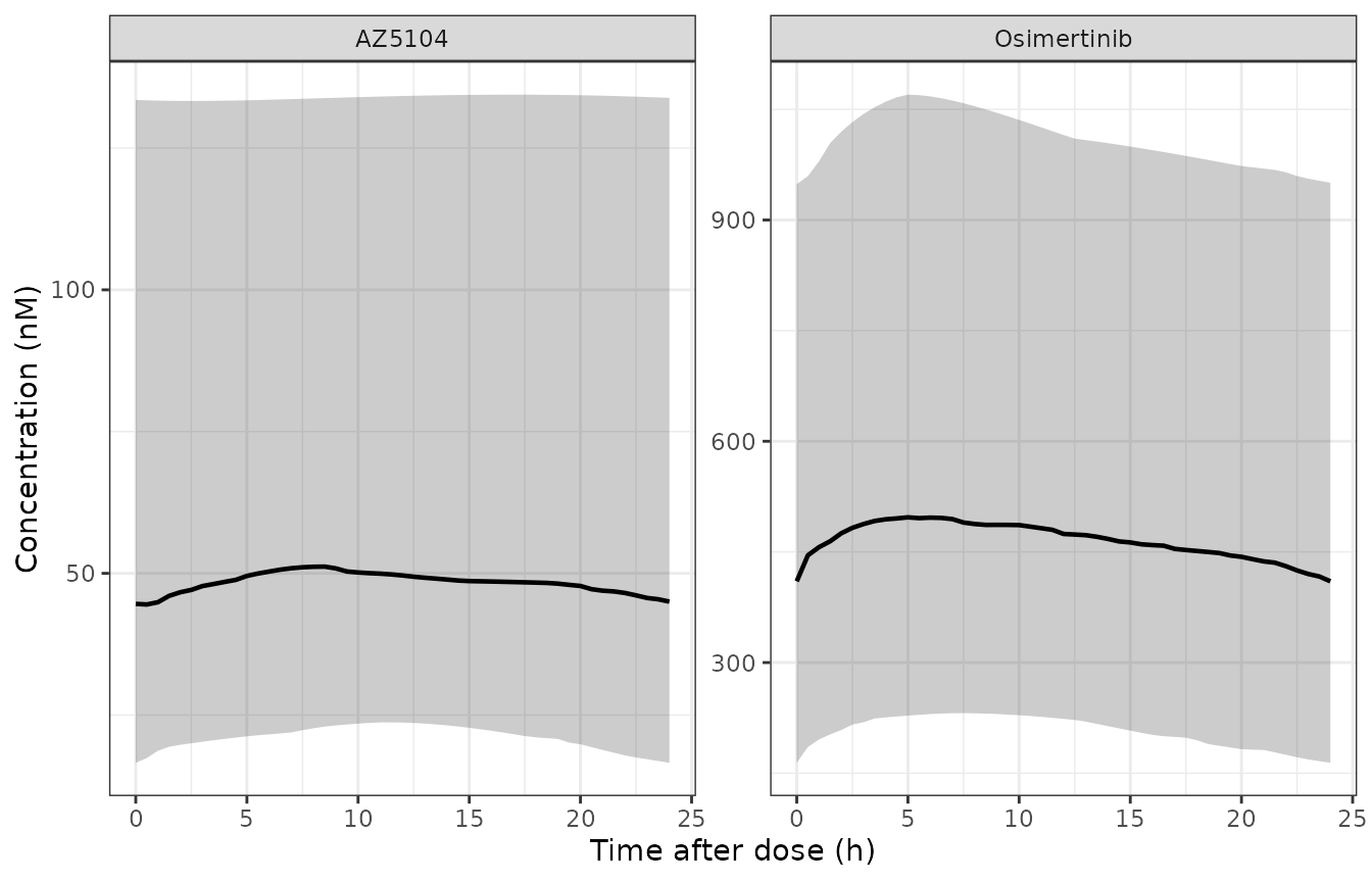
Simulated steady-state osimertinib and AZ5104 concentration-time profiles over the final 24 h dosing interval (200 virtual patients; median and 5th-95th percentile band). Compare with Yang 2025 Figure 2, which plots the observed concentrations across the six pooled studies.
Structural verification
Closed-form mass balance
At steady state the AUC over one dosing interval must equal dose
divided by apparent clearance, with the dose converted to nmol using
each analyte’s own molecular weight – exactly the convention the control
stream’s S2 and S3 encode. Both sides use the
same parameters here, so the only difference is numerical integration
error and the bound is tight.
MW_parent <- 499.61
MW_az5104 <- 485.59

trapz <- function(t, y) sum(diff(t) * (head(y, -1) + tail(y, -1)) / 2)

ref_ss <- sim_ref |> dplyr::filter(time >= ss_start) |> dplyr::arrange(time)
auc_parent_solved <- trapz(ref_ss$time, ref_ss$Cc)
auc_metab_solved  <- trapz(ref_ss$time, ref_ss$Cc_az5104)

auc_parent_closed <- (dose_amt * 1e-3 / MW_parent * 1e9) / 14.3452
auc_metab_closed  <- (0.25 * dose_amt * 1e-3 / MW_az5104 * 1e9) / 32.0484

tibble::tibble(
  Analyte       = c("Osimertinib", "AZ5104"),
  `Solved AUCtau (nM*h)` = round(c(auc_parent_solved, auc_metab_solved), 1),
  `Closed form (nM*h)`   = round(c(auc_parent_closed, auc_metab_closed), 1),
  `Difference (%)`       = round(100 * c(auc_parent_solved / auc_parent_closed,
                                         auc_metab_solved  / auc_metab_closed) - 100, 3)
)
#> # A tibble: 2 × 4
#>   Analyte     `Solved AUCtau (nM*h)` `Closed form (nM*h)` `Difference (%)`
#>   <chr>                        <dbl>                <dbl>            <dbl>
#> 1 Osimertinib                  11160               11162.           -0.02
#> 2 AZ5104                        1285                1285.           -0.014
stopifnot(
  abs(auc_parent_solved / auc_parent_closed - 1) < 0.005,
  abs(auc_metab_solved  / auc_metab_closed  - 1) < 0.005
)
This gate is what proves the metabolite transfer convention. The control stream moves amount from the central to the metabolite compartment 1:1, with no molar stoichiometric correction, and only then forms the metabolite concentration using the AZ5104 molecular weight. Inserting a molar correction would scale AZ5104 exposure by 0.9719 and break this identity.
Time to peak
Yang 2025 Results reports model-derived steady-state tmax medians of 6.7 h (IQR 5.9-7.4) for osimertinib and 11.3 h (IQR 9.9-12.5) for AZ5104. These are model-derived, so the typical-value profile should land on them. Note this is not the same quantity as the Table S5 observed NCA tmax (4.50 h and 4.00 h), which is bounded by a sparse sampling grid that stopped at 6 h post-dose.
tmax_parent <- ref_ss$time[which.max(ref_ss$Cc)] - ss_start
tmax_metab  <- ref_ss$time[which.max(ref_ss$Cc_az5104)] - ss_start

tibble::tibble(
  Analyte             = c("Osimertinib", "AZ5104"),
  `Typical tmax (h)`  = c(tmax_parent, tmax_metab),
  `Yang 2025 median`  = c(6.7, 11.3),
  `Yang 2025 IQR`     = c("5.9-7.4", "9.9-12.5")
)
#> # A tibble: 2 × 4
#>   Analyte     `Typical tmax (h)` `Yang 2025 median` `Yang 2025 IQR`
#>   <chr>                    <dbl>              <dbl> <chr>
#> 1 Osimertinib                7                  6.7 5.9-7.4
#> 2 AZ5104                    11.5               11.3 9.9-12.5
# Deterministic typical-value profile; must fall inside the published IQR.
stopifnot(
  tmax_parent >= 5.9, tmax_parent <= 7.4,
  tmax_metab  >= 9.9, tmax_metab  <= 12.5
)
Half-lives
thalf_parent <- log(2) * 1151.11 / 14.3452
thalf_metab  <- log(2) * 151.014 / 32.0484
tibble::tibble(
  Analyte              = c("Osimertinib", "AZ5104"),
  `Typical t1/2 (h)`   = round(c(thalf_parent, thalf_metab), 1),
  `Yang 2025 median`   = c(47.7, 3.1),
  `Yang 2025 IQR`      = c("31.8-69.0", "2.2-4.5")
)
#> # A tibble: 2 × 4
#>   Analyte     `Typical t1/2 (h)` `Yang 2025 median` `Yang 2025 IQR`
#>   <chr>                    <dbl>              <dbl> <chr>
#> 1 Osimertinib               55.6               47.7 31.8-69.0
#> 2 AZ5104                     3.3                3.1 2.2-4.5
stopifnot(
  thalf_parent > 31.8, thalf_parent < 69.0,
  thalf_metab  >  2.2, thalf_metab  <  4.5
)
AZ5104’s own elimination half-life is far shorter than the parent’s, so the metabolite is formation-rate limited and its observed decline tracks osimertinib.
Replicating Figure 3 (covariate forest plot)
Yang 2025 Results quotes two exact numbers off its own forest plot: “The ratio of AZ5104 exposures for high body weight (89 kg) and for low body weight (43 kg) vs. the reference population was 0.76 and 1.31, respectively” (the published sentence has a typographical “AZ5102”). Because AZ5104 steady-state AUC is inversely proportional to CLm/F, and weight enters CLm/F only through the 0.740376 power term, these are a closed-form two-point test of that exponent.
wt_ratio <- function(wt) (wt / 62)^-0.740376
fp <- tibble::tibble(
  `Body weight (kg)`        = c(89, 43),
  Percentile                = c("95th", "5th"),
  `Model AZ5104 AUCss ratio` = round(wt_ratio(c(89, 43)), 3),
  `Yang 2025 Results`        = c(0.76, 1.31)
)
fp
#> # A tibble: 2 × 4
#>   `Body weight (kg)` Percentile `Model AZ5104 AUCss ratio` `Yang 2025 Results`
#>                <dbl> <chr>                           <dbl>               <dbl>
#> 1                 89 95th                            0.765                0.76
#> 2                 43 5th                             1.31                 1.31
# Closed-form against a printed number: exact to the paper's 2 decimal places.
stopifnot(all(abs(wt_ratio(c(89, 43)) - c(0.76, 1.31)) < 0.01))
The full simulated forest plot, over each retained covariate at the 5th and 95th percentile (or against the White reference for race), reproduces the shape of Figure 3 – every effect sits inside or close to the 0.8-1.25 bioequivalence band, which is the paper’s basis for calling none of them clinically meaningful:
q05_wt <- 43; q95_wt <- 89; q05_alb <- 31; q95_alb <- 47

# AUCss ratios are inverse-clearance ratios; Cmaxss additionally moves with volume.
eff <- tibble::tribble(
  ~Covariate,                  ~Analyte,      ~ratio,
  "Weight 43 kg (5th)",        "Osimertinib", (q05_wt/62)^-0.359774,
  "Weight 89 kg (95th)",       "Osimertinib", (q95_wt/62)^-0.359774,
  "Albumin 31 g/L (5th)",      "Osimertinib", (q05_alb/40)^-0.674479,
  "Albumin 47 g/L (95th)",     "Osimertinib", (q95_alb/40)^-0.674479,
  "Weight 43 kg (5th)",        "AZ5104",      (q05_wt/62)^-0.740376,
  "Weight 89 kg (95th)",       "AZ5104",      (q95_wt/62)^-0.740376,
  "Albumin 31 g/L (5th)",      "AZ5104",      (q05_alb/40)^-0.722460,
  "Albumin 47 g/L (95th)",     "AZ5104",      (q95_alb/40)^-0.722460,
  "Asian other vs White",      "AZ5104",      1 / (1 + 0.161274),
  "Japanese vs White",         "AZ5104",      1 / (1 + 0.181966)
)

ggplot2::ggplot(eff, ggplot2::aes(ratio, Covariate)) +
  ggplot2::annotate("rect", xmin = 0.8, xmax = 1.25, ymin = -Inf, ymax = Inf,
                    alpha = 0.15, fill = "darkred") +
  ggplot2::geom_vline(xintercept = 1, linetype = "dashed") +
  ggplot2::geom_point(size = 2.5) +
  ggplot2::facet_wrap(~Analyte, scales = "free_y") +
  ggplot2::labs(x = "AUCss ratio vs reference patient", y = NULL) +
  ggplot2::theme_bw()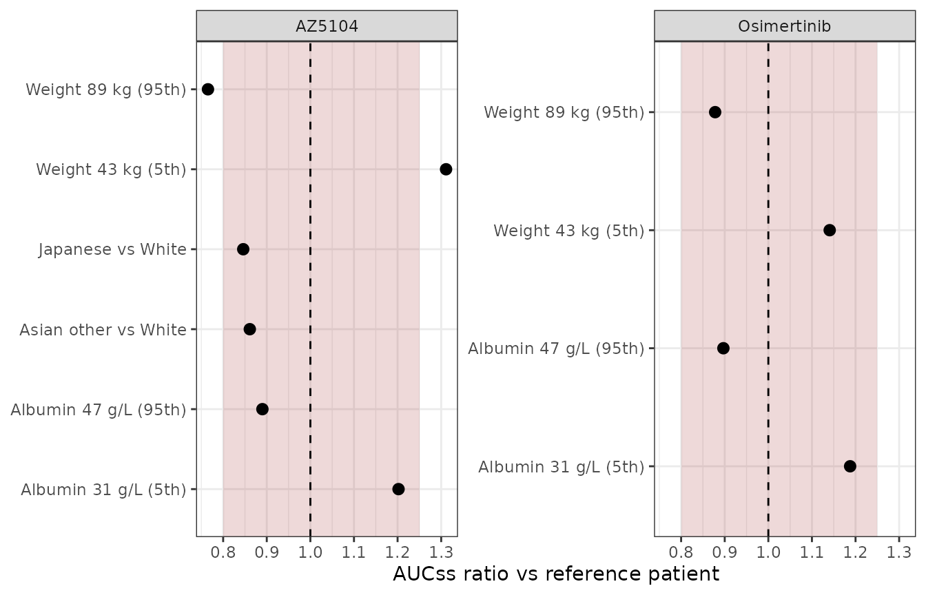
Covariate effects on steady-state exposure relative to the reference patient (White, 62 kg, albumin 40 g/L). Replicates Yang 2025 Figure 3. The shaded band is the 0.80-1.25 bioequivalence reference range.
# Directional content of Figure 3: heavier patients and higher albumin both
# clear faster, so both reduce exposure; the two retained race effects raise
# metabolite clearance and so reduce AZ5104 exposure.
stopifnot(
  (q95_wt/62)^-0.359774  < 1, (q05_wt/62)^-0.359774  > 1,
  (q95_alb/40)^-0.674479 < 1, (q05_alb/40)^-0.674479 > 1,
  1 / (1 + 0.161274) < 1, 1 / (1 + 0.181966) < 1
)
PKNCA validation
Steady-state NCA over the final 24 h dosing interval, for both analytes, in nM.
nca_frame <- function(conc_col) {
  sim |>
    dplyr::filter(time >= ss_start, !is.na(.data[[conc_col]])) |>
    dplyr::transmute(id, time = time - ss_start, conc = .data[[conc_col]],
                     treatment = "Osimertinib 80 mg QD")
}

conc_parent <- nca_frame("Cc")
conc_metab  <- nca_frame("Cc_az5104")

dose_df <- tibble::tibble(id = unique(conc_parent$id), time = 0,
                          amt = dose_amt, treatment = "Osimertinib 80 mg QD")

intervals <- data.frame(start = 0, end = 24,
                        cmax = TRUE, tmax = TRUE, cmin = TRUE,
                        auclast = TRUE, cav = TRUE)

dose_obj <- PKNCA::PKNCAdose(dose_df, amt ~ time | treatment + id, doseu = "mg")

nca_parent <- PKNCA::pk.nca(PKNCA::PKNCAdata(
  PKNCA::PKNCAconc(conc_parent, conc ~ time | treatment + id,
                   concu = "nmol/L", timeu = "h"),
  dose_obj, intervals = intervals))

nca_metab <- PKNCA::pk.nca(PKNCA::PKNCAdata(
  PKNCA::PKNCAconc(conc_metab, conc ~ time | treatment + id,
                   concu = "nmol/L", timeu = "h"),
  dose_obj, intervals = intervals))
Comparison against published NCA
Yang 2025 Table S5 reports observed steady-state NCA for the FLAURA2 osimertinib-plus-chemotherapy arm (N = 244), as geometric means.
simulated <- dplyr::bind_rows(
  as.data.frame(nca_parent$result) |> dplyr::mutate(analyte = "Osimertinib"),
  as.data.frame(nca_metab$result)  |> dplyr::mutate(analyte = "AZ5104")
)

reference <- tibble::tribble(
  ~analyte,      ~auclast, ~cmax,  ~cmin,
  "Osimertinib",    11840, 587.5,  392.5,
  "AZ5104",          1277,  59.07,  45.51
)

cmp <- nlmixr2lib::ncaComparisonTable(
  simulated     = simulated,
  reference     = reference,
  by            = "analyte",
  params        = c("auclast", "cmax", "cmin"),
  units         = c(auclast = "nmol*h/L", cmax = "nmol/L", cmin = "nmol/L"),
  tolerance_pct = 20
)

knitr::kable(cmp, caption = paste(
  "Simulated steady-state NCA vs Yang 2025 Table S5 observed geometric means",
  "(FLAURA2 osimertinib plus chemotherapy arm, N = 244).",
  "* marks a difference greater than 20%."
))| NCA parameter | analyte | Reference | Simulated | % diff |
|---|---|---|---|---|
| Cmax (nmol/L) | Osimertinib | 588 | 488 | -17.0% |
| Cmax (nmol/L) | AZ5104 | 59.1 | 47.7 | -19.2% |
| Cmin (nmol/L) | Osimertinib | 392 | 391 | -0.4% |
| Cmin (nmol/L) | AZ5104 | 45.5 | 42.1 | -7.4% |
| AUClast (nmol*h/L) | Osimertinib | 11800 | 10800 | -8.9% |
| AUClast (nmol*h/L) | AZ5104 | 1280 | 1080 | -15.5% |
# Structural gate on the centre of the distribution. A mis-transcribed
# clearance, dose or molecular weight moves these by tens of percent.
auc_p <- simulated |> dplyr::filter(analyte == "Osimertinib", PPTESTCD == "auclast")
auc_m <- simulated |> dplyr::filter(analyte == "AZ5104",      PPTESTCD == "auclast")
stopifnot(
  abs(median(auc_p$PPORRES) / 11840 - 1) < 0.25,
  abs(median(auc_m$PPORRES) /  1277 - 1) < 0.25
)
The metabolite-to-parent exposure ratio is an internally consistent check that does not depend on either analyte’s absolute calibration:
mr_auc <- median(auc_m$PPORRES) / median(auc_p$PPORRES)
tibble::tibble(
  Metric               = "MRAUCss (AZ5104 / osimertinib)",
  Simulated            = round(mr_auc, 4),
  `Yang 2025 Table S5` = 0.1078
)
#> # A tibble: 1 × 3
#>   Metric                         Simulated `Yang 2025 Table S5`
#>   <chr>                              <dbl>                <dbl>
#> 1 MRAUCss (AZ5104 / osimertinib)     0.100                0.108
stopifnot(abs(mr_auc / 0.1078 - 1) < 0.30)
Assumptions and deviations
The albumin effect on AZ5104 volume is negative. Table 2 prints its magnitude (0.65) without a sign, and prints its bootstrap CI with the bounds reversed (“0.68 (1.28-0.42)”). Equation 5 and
$THETA(13) = -0.652465both carry the negative sign and are taken as authoritative.Table 2’s between-subject-variability column is on the variance scale. This is confirmed by the control stream’s
$OMEGAvalues and, independently, by back-transforming to the paper’s own published %CV figures (chunkomega_scaleabove). The$OMEGA BLOCK(2)off-diagonal is a covariance, not the correlation coefficient its Table 2 row label implies.Race coefficients are on a
(1 + theta)fractional-deviation form, not a power or exponential form. Table 2 lists 0.16 and 0.18; Equation 4 writes the corresponding multipliers as 1.16 and 1.18; the control stream’sCLM1ETHLblock computes1 + THETA(n). Note this differs from the siblingBrown_2017_osimertinibmodel only in the estimated values, not the form.Chinese and Other race indicators are retained with coefficients fixed at zero. Backward elimination found both non-significant (Table S2) and the final control stream holds
$THETA(15)and$THETA(17)at0 FIX. They are kept in the model file so the covariate screen stays auditable; they have no numerical effect.The parent-to-metabolite transfer carries no molar stoichiometric correction. Amount moves 1:1 and each analyte’s concentration is then formed with its own molecular weight, per
S2andS3. This is a deliberate departure fromBrown_2017_osimertinib, which applies an explicitmw_az5104 / mw_parentfactor in its ODE. Yang 2025’s convention is what its own control stream fits, and it is what reproduces the Table S5 AZ5104 exposure (to 0.6%, versus about 3% low with a molar correction).Concentrations are in nM, not mg/L, following the source throughout (assay ranges, additive residual errors, AUCss quartiles and Table S5 are all nM).
Brown_2017_osimertinibuses mg/L and converts in its vignette; the two models are therefore not directly comparable without unit conversion.Missing-covariate handling is not reproduced. The control stream maps a missing weight or albumin (coded
-999) onto a covariate factor of 1. This model expects observed values; Table 1 reports missingness of 0.4% for weight and 1.1% for albumin, so the effect on any simulation is negligible.The cohort’s covariate marginals are drawn independently. Yang 2025 does not report the weight-albumin correlation or the joint distribution by race, so weight, albumin and race are sampled independently from the Table 1 marginals. This widens the simulated exposure spread slightly relative to the real population.
Cmax is compared on
Cc(without residual error). Table S5’s Cmax is an observed geometric mean from a sparse grid (pre-dose and 1, 2, 4 and 6 h at C3D1) that cannot resolve the model’s 6.7 h median tmax, so the observed and model-derived peak quantities are not strictly the same measurement. The parent Cmax accordingly sits below the Table S5 value; AUC, which is far less sensitive to grid density, agrees closely.
Not extracted: the exposure-response analyses
Yang 2025’s second half is an exposure-response assessment of the FLAURA2 combination arm. It is deliberately not part of this model file, for two reasons.
The efficacy analysis is a Cox proportional-hazards model of progression-free survival. A Cox model is semi-parametric: it estimates covariate coefficients against an unspecified baseline hazard that is never estimated or published. Tables S3 and S4 report only minimum -2LL, likelihood differences and p-values – no hazard-ratio coefficients and no baseline hazard – so there is nothing that could be encoded as a simulable time-to-event model without inventing a baseline hazard function.
The safety analysis is a set of logistic regressions of adverse-event occurrence against exposure quartiles, reported graphically in Figure 5 with no tabulated intercepts or slopes.
In any case both analyses are negative findings. No osimertinib or AZ5104 exposure metric (AUCss, Cmaxss, Cminss) was significant for PFS; the only retained covariate was the number of pemetrexed cycles, which the authors themselves caution is confounded by survivorship bias. No exposure-safety relationship was found either, apart from an inverse association with AEs leading to dose reduction that the paper interprets as non-causal. There is therefore no drug-effect relationship to encode.