Isoniazid antimycobacterial pharmacodynamics (Cordes 2016)
Source:vignettes/articles/Cordes_2016_isoniazid.Rmd
Cordes_2016_isoniazid.RmdModel and source
Cordes 2016 couples a whole-body physiologically based pharmacokinetic (PBPK) model of isoniazid (INH) and six of its metabolites to a pharmacodynamic (PD) model of Mycobacterium tuberculosis killing in the human lung, and uses the combination to argue for NAT2-acetylator-specific dose adjustment.
- Article: https://doi.org/10.1128/AAC.00508-16
mod <- rxode2::rxode(readModelDb("Cordes_2016_isoniazid_pd"))
cat(mod$reference, "\n")
#> Cordes H, Thiel C, Aschmann HE, Baier V, Blank LM, Kuepfer L. (2016). A physiologically based pharmacokinetic model of isoniazid and its application in individualizing tuberculosis chemotherapy. Antimicrobial Agents and Chemotherapy 60(10):6134-6145. doi:10.1128/AAC.00508-16.
What this package carries, and what it does not
This package carries the PD half only, as
Cordes_2016_isoniazid_pd. That is a deliberate scope
decision, not an oversight, and the reason is worth stating plainly
because it determines how the model must be used.
The drug input in Cordes 2016 is a whole-body PBPK model built in
PK-Sim 6.0.3, a proprietary platform. The paper
publishes the compound card (Table 1: molecular weight, log P,
fraction unbound, pKa, solubility) and the kinetic
card (Table 2 and supplementary Table S1: Michaelis-Menten
Vmax and Km for eight metabolic, transport and
excretion reactions). It does not publish the two
things that would be needed to rebuild the distribution model outside
the platform:
- Tissue:plasma partition coefficients. These are computed inside PK-Sim from the physicochemistry by a named method (“used to parameterize the basic distribution model in PK-Sim”, Materials and Methods). No coefficient is printed, and the paper does not state which of the platform’s partitioning variants was selected. (The two occurrences of “Kp” in the paper are the Table 1 footnote glossing log P as a partition coefficient - octanol/water lipophilicity, not a tissue coefficient.)
-
Tissue-specific enzyme and transporter abundances.
“Tissue specific relative enzyme and transporter abundances were
quantified by gene expression data provided by the PBPK modeling
software” (supplement). The
Vmaxvalues in Table 2 are per-volume rates that the platform redistributes across organs using that unpublished expression profile, so they cannot be applied without it.
No PK-Sim project file is deposited; the supplement is a PDF plus two spreadsheets. Supplementary Table S2 does deposit the full 1,000-individual population anatomy and physiology export (organ volumes, specific blood flow rates, tissue-composition fractions), which is more than most platform papers provide - but that is the borrowed, human-physiology half of a PBPK model. It certifies only itself; none of the drug-specific half is in it.
Nor is there a reduced compartmental model to fall back on. The paper reports no clearance value, no volume of distribution, no AUC and no Cmax anywhere in the text, tables or supplement, so there is nothing from which even a one-compartment INH model could be recovered.
The PD half, by contrast, is completely specified: equations 1-3 are
printed, and all seven parameters are given in Table 5. Exposure
therefore enters this file as the externally supplied covariate
CEFFECT, on the same pattern as
Gao_2025_cefquinome_pkpd_index and
Crass_2025_pegcetacoplan_ga_exposureresponse.
Population
The PD parameters Emax, Km and
h were fitted to early bactericidal activity (EBA) measured
in sputum from NAT2-phenotype-specific pulmonary tuberculosis patients
over the first two days of INH monotherapy, pooled from Donald 1997
(Am J Respir Crit Care Med 156:895-900, reference 23) and
Donald 2004 (Clin Infect Dis 39:1425-1430, reference 45). The
supplement records that only patient subgroups with more than three
individuals were used, to limit the influence of outliers, and that the
original studies’ sampling patterns were reproduced in simulation. QD
doses from 9 mg to 600 mg are represented (Figure 5B).
The growth rate mu and the immune killing rate
beta0 were not fitted. They come from a
literature review of M. tuberculosis growth rates in untreated
humans and in immunocompetent versus immune-deficient mice (supplement
equations A2-A3).
knitr::kable(
  tibble::tibble(
    Item = c("Species", "Disease state", "PD calibration data", "Dose range in calibration",
             "Growth / immune rates", "Variability"),
    Value = c(
      "Human",
      "Active pulmonary tuberculosis",
      "EBA in sputum, first 2 days of INH monotherapy (Donald 1997; Donald 2004)",
      "9 mg to 600 mg QD",
      "Literature-derived, not fitted (supplement A2-A3)",
      "None reported for the PD layer; deterministic typical-value model"
    )
  )
)| Item | Value |
|---|---|
| Species | Human |
| Disease state | Active pulmonary tuberculosis |
| PD calibration data | EBA in sputum, first 2 days of INH monotherapy (Donald 1997; Donald 2004) |
| Dose range in calibration | 9 mg to 600 mg QD |
| Growth / immune rates | Literature-derived, not fitted (supplement A2-A3) |
| Variability | None reported for the PD layer; deterministic typical-value model |
Cordes 2016’s population work simulated 1,000 virtual individuals per acetylator phenotype, but that variability lives entirely in the PBPK layer (anatomy and physiology, supplementary Table S2) and is therefore not represented here.
Source trace
Every value in ini() and every equation in
model(), with its source location.
knitr::kable(
  tibble::tribble(
    ~Quantity, ~Value, ~Source,
    "mu (growth, no immune contribution)", "0.0428 log10 CFU/day", "Supplement eq. A2 (NOT Table 5; see Errata)",
    "beta0 (immune killing)", "0.0219 log10 CFU/day", "Table 5; supplement eq. A3",
    "Emax (max INH killing)", "0.534 log10 CFU/day", "Table 5, Fitted",
    "Km -> ec50 (half-max C/MIC)", "25.19 (multiples of MIC)", "Table 5, Fitted (units; see Errata)",
    "h (Hill coefficient)", "0.56", "Table 5, Fitted",
    "MIC", "1.46 umol/L", "Table 5, from reference 41 (Schon 2009); = 0.2 mg/L / 137.14 g/mol",
    "N0 (initial burden)", "10 log10 CFU/L", "Table 5, 'Arbitrary'",
    "d -> f_immune", "1 (immunocompetent)", "Materials and Methods: beta* = beta0 * d, d in [0, 1]",
    "gamma (sigmoid Emax)", "Emax*(C/MIC)^h / (Km^h + (C/MIC)^h)", "Equation 2 (after Czock & Keller 2007, ref. 47)",
    "dN/dt", "mu - beta0*d - gamma", "Equation 3 and supplement eq. A1",
    "CEFFECT", "Unbound INH, lung interstitium", "Results, 'PBPK/PD model development'"
  )
)| Quantity | Value | Source |
|---|---|---|
| mu (growth, no immune contribution) | 0.0428 log10 CFU/day | Supplement eq. A2 (NOT Table 5; see Errata) |
| beta0 (immune killing) | 0.0219 log10 CFU/day | Table 5; supplement eq. A3 |
| Emax (max INH killing) | 0.534 log10 CFU/day | Table 5, Fitted |
| Km -> ec50 (half-max C/MIC) | 25.19 (multiples of MIC) | Table 5, Fitted (units; see Errata) |
| h (Hill coefficient) | 0.56 | Table 5, Fitted |
| MIC | 1.46 umol/L | Table 5, from reference 41 (Schon 2009); = 0.2 mg/L / 137.14 g/mol |
| N0 (initial burden) | 10 log10 CFU/L | Table 5, ‘Arbitrary’ |
| d -> f_immune | 1 (immunocompetent) | Materials and Methods: beta* = beta0 * d, d in [0, 1] |
| gamma (sigmoid Emax) | Emax*(C/MIC)^h / (Km^h + (C/MIC)^h) | Equation 2 (after Czock & Keller 2007, ref. 47) |
| dN/dt | mu - beta0*d - gamma | Equation 3 and supplement eq. A1 |
| CEFFECT | Unbound INH, lung interstitium | Results, ‘PBPK/PD model development’ |
Dimensional analysis
N is a burden on the log10 CFU/L scale and every rate
term is in log10 CFU/day, so equation 3 is a balance of like
quantities:
| Term | Units |
|---|---|
mu |
log10 CFU / day |
beta0 * f_immune |
log10 CFU / day (f_immune unitless) |
CEFFECT / mic |
unitless (umol/L over umol/L) |
ec50^hill, (CEFFECT/mic)^hill
|
unitless |
gamma |
log10 CFU / day (emax scales a unitless fraction) |
knet |
log10 CFU / day |
The model file integrates the state on the linear
CFU/L scale as d/dt(bact) = ln(10) * knet * bact, which
makes log10(bact) change by exactly knet per
day. The check below confirms that identity numerically rather than
asserting it in prose.
Structural validation
There is no dose and no absorption-distribution-elimination profile in this model, so non-compartmental analysis is not an applicable validation and PKNCA is deliberately not used here. The checks below are the mechanistic-model equivalents: exact rate identities, a saturation limit, and the integrator identity. All are deterministic - there is no simulated cohort and no drawn random effect anywhere in this vignette - so exact tolerances are appropriate and are used.
# Solve the PD model at a clamped (constant) effect-site concentration and
# return the realised net rate of change of log10(burden), in log10 CFU/day.
knet_at <- function(ceffect, f_immune = 1, days = 2) {
  ev <- as.data.frame(rxode2::et(seq(0, days, by = 0.05)))
  ev$CEFFECT <- ceffect
  s <- rxode2::rxSolve(mod, ev, params = c(f_immune = f_immune),
                       returnType = "data.frame")
  stats::coef(stats::lm(log10(s$bact) ~ s$time))[[2]]
}
1. Untreated growth reproduces the literature-derived rates
With no drug, the model must reproduce the two growth rates the
supplement derives from the literature: mu - beta0 = 0.0209
log10 CFU/day for an untreated immunocompetent patient,
and mu = 0.0428 log10 CFU/day when the immune contribution
is fully removed.
untreated_ic <- knet_at(0, f_immune = 1)
untreated_id <- knet_at(0, f_immune = 0)

stopifnot(
  isTRUE(all.equal(untreated_ic, 0.0209, tolerance = 1e-6)),
  isTRUE(all.equal(untreated_id, 0.0428, tolerance = 1e-6))
)

tibble::tibble(
  Scenario = c("Untreated, immunocompetent", "Untreated, fully immune-deficient"),
  Simulated = c(untreated_ic, untreated_id),
  Published = c(0.0209, 0.0428),
  Source = c("Supplement, mu(MT)_IC^human", "Supplement eq. A2, mu(MT)_ID^human")
) |>
knitr::kable(digits = 5)| Scenario | Simulated | Published | Source |
|---|---|---|---|
| Untreated, immunocompetent | 0.0209 | 0.0209 | Supplement, mu(MT)_IC^human |
| Untreated, fully immune-deficient | 0.0428 | 0.0428 | Supplement eq. A2, mu(MT)_ID^human |
This is the check that pins the mu value. It is the
reason this file uses 0.0428 rather than the 0.048 printed in Table 5:
with 0.048 the untreated immunocompetent rate would be 0.0261,
contradicting the supplement’s own literature-derived 0.0209. The
assertion below states that explicitly so the choice is mechanically
gated rather than argued in prose.
mu_used <- exp(mod$theta[["lkgrowth"]])
beta0_used <- exp(mod$theta[["lkimm"]])

stopifnot(
  # The supplement's three rates are mutually exact: A3 says
  # beta^human = mu_ID - mu_IC, i.e. 0.0219 = 0.0428 - 0.0209.
  isTRUE(all.equal(mu_used - beta0_used, 0.0209, tolerance = 1e-9)),
  # Table 5's printed mu = 0.048 does NOT satisfy that identity.
  !isTRUE(all.equal(0.048 - beta0_used, 0.0209, tolerance = 1e-3))
)
2. Half-maximal effect sits at the fitted ec50
At C = ec50 * MIC the sigmoid must deliver exactly half
of Emax, so the net rate must be
0.0209 - Emax/2.
emax_used <- exp(mod$theta[["lemax"]])
ec50_used <- exp(mod$theta[["lec50"]])
mic_used <- mod$theta[["mic"]]

half_max <- knet_at(ec50_used * mic_used, f_immune = 1)

stopifnot(
  isTRUE(all.equal(half_max, 0.0209 - emax_used / 2, tolerance = 1e-6))
)

c(simulated = half_max, expected = 0.0209 - emax_used / 2)
#> simulated  expected
#>   -0.2461   -0.2461
3. Saturating exposure approaches the Emax limit
As C grows the kill rate must approach
Emax, so the net rate must approach
0.0209 - 0.534 = -0.5131 log10 CFU/day from above and never
cross it.
sat <- vapply(c(1e3, 1e5, 1e7, 1e9), knet_at, numeric(1))
limit <- 0.0209 - emax_used

stopifnot(
  all(sat > limit), # never crosses the asymptote
  all(diff(sat) < 0), # monotone approach
  sat[length(sat)] < limit + 0.01 # gets there
)

tibble::tibble(`CEFFECT (umol/L)` = c(1e3, 1e5, 1e7, 1e9), `knet` = sat) |>
knitr::kable(digits = 5)| CEFFECT (umol/L) | knet |
|---|---|
| 1e+03 | -0.44052 |
| 1e+05 | -0.50680 |
| 1e+07 | -0.51262 |
| 1e+09 | -0.51306 |
The saturated EBA of 0.513 log10 CFU/day is the right size for
isoniazid, whose measured 2-day EBA is in the region of 0.5 log10
CFU/day - one of the three lines of evidence recorded in the model file
for dropping the N0 factor that equation 3 prints (see
Errata).
4. The integrator identity holds
log10(bact) must fall on a straight line of slope
knet, because dN/dt does not depend on
N.
ev <- as.data.frame(rxode2::et(seq(0, 2, by = 0.05)))
ev$CEFFECT <- 30
s <- rxode2::rxSolve(mod, ev, returnType = "data.frame")
fit <- stats::lm(log10(s$bact) ~ s$time)

# The closed form of equation 3 at a clamped concentration, evaluated in plain
# R independently of rxode2. The solved slope must reproduce it.
hill_used <- exp(mod$theta[["lhill"]])
c_mic <- 30 / mic_used
knet_closed <- 0.0209 - emax_used * c_mic^hill_used /
  (ec50_used^hill_used + c_mic^hill_used)

stopifnot(
  # A straight line, to the solver's tolerance.
  max(abs(stats::residuals(fit))) < 1e-5,
  # It starts exactly at the declared N0.
  isTRUE(all.equal(log10(s$bact[1]), 10, tolerance = 1e-9)),
  # And its slope is the closed-form net rate, not merely some constant.
  isTRUE(all.equal(stats::coef(fit)[[2]], knet_closed, tolerance = 1e-7))
)

c(
  max_residual = max(abs(stats::residuals(fit))),
  solved_slope = stats::coef(fit)[[2]],
  closed_form = knet_closed
)
#>  max_residual  solved_slope   closed_form
#>  2.312022e-07 -2.308889e-01 -2.308889e-01
The isoniazid killing sigmoid
Reproducing equation 2 across the exposure range, which is the shape the paper fitted to the EBA data.
sig <- tibble::tibble(c_mic = 10^seq(-1, 4, length.out = 200)) |>
  mutate(gamma = emax_used * c_mic^exp(mod$theta[["lhill"]]) /
    (ec50_used^exp(mod$theta[["lhill"]]) + c_mic^exp(mod$theta[["lhill"]])))

ggplot(sig, aes(c_mic, gamma)) +
  geom_line(linewidth = 0.8) +
  geom_hline(yintercept = emax_used / 2, linetype = "dashed", colour = "grey40") +
  geom_vline(xintercept = ec50_used, linetype = "dashed", colour = "grey40") +
  scale_x_log10() +
  labs(
    x = "C / MIC (unitless)",
    y = expression(gamma ~ "(log10 CFU/day)"),
    title = "Cordes 2016 equation 2"
  ) +
  theme_bw()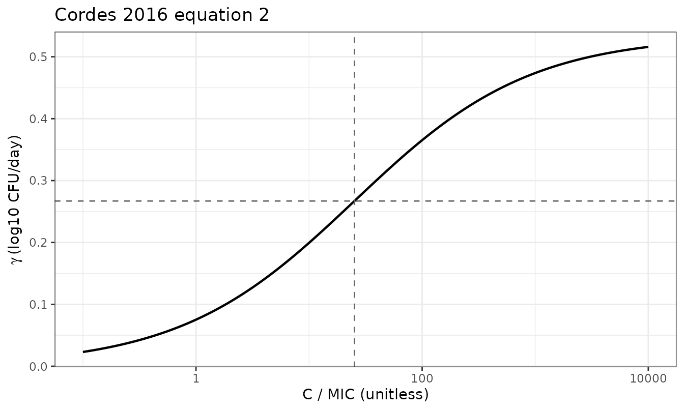
Isoniazid-induced killing rate (equation 2) against exposure, expressed as multiples of the MIC. The dashed lines mark the fitted ec50 and half of Emax.
The Hill coefficient of 0.56 is well below 1, so the curve is shallow: exposure has to rise by orders of magnitude to move the kill rate appreciably. That shallowness is what drives the paper’s central finding - a fast acetylator cannot simply be dosed up to a slow acetylator’s efficacy.
Net effect of exposure and immune status
grid <- tidyr::expand_grid(
  ceffect = 10^seq(-1, 3, length.out = 60),
  f_immune = c(0, 0.25, 0.5, 1)
) |>
  rowwise() |>
  mutate(knet = knet_at(ceffect, f_immune)) |>
  ungroup()

ggplot(grid, aes(ceffect, knet, colour = factor(f_immune))) +
  geom_line(linewidth = 0.8) +
  geom_hline(yintercept = 0, linetype = "dotted") +
  scale_x_log10() +
  labs(
    x = "Unbound isoniazid in lung interstitium (umol/L)",
    y = "Net rate (log10 CFU/day)",
    colour = "f_immune",
    title = "Exposure-response by immune status"
  ) +
  theme_bw()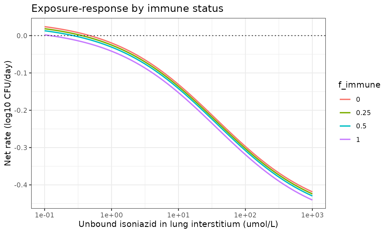
Net rate of change of mycobacterial burden against isoniazid exposure, at four levels of host immune competence. Below the zero line the burden falls.
Immune deficiency shifts the whole curve upward by up to
beta0 = 0.0219 log10 CFU/day, reproducing the paper’s
qualitative claim that immune-deficient patients achieve lower treatment
efficacy at any given dose. The claim is asserted, not just plotted:
Chaining an isoniazid PK model to the PD model
Because Cordes 2016’s own PBPK layer cannot be ported (above), the
natural way to exercise this model is to drive CEFFECT with
a published INH population PK model.
Vinnard_2017_isoniazid, already in this library, is a
NAT2-aware two-compartment oral model, which makes it a reasonable
stand-in for testing the paper’s acetylator argument.
This is an illustration, not a replication. Vinnard 2017 is a different study in a different population, and its plasma concentrations are not Cordes 2016’s PBPK lung-interstitial concentrations. The numbers below will not match Cordes 2016’s published efficacy percentages and are not intended to.
The plasma-to-effect-site step uses two values from Cordes 2016 itself: the INH fraction unbound of 0.90 (Table 1) and the molecular weight of 137.14 g/mol (Table 1). The paper’s Discussion justifies treating unbound plasma as a proxy for the lung interstitium, citing evidence that INH concentrations in plasma, epithelial lining fluid and alveolar cells do not differ significantly.
pk <- rxode2::rxode(readModelDb("Vinnard_2017_isoniazid"))
#> Warning: some etas defaulted to non-mu referenced, possible parsing error: etaiov_cl_1, etaiov_cl_2
#> as a work-around try putting the mu-referenced expression on a simple line
pk_typ <- rxode2::zeroRe(pk)
#> Warning: some etas defaulted to non-mu referenced, possible parsing error: etaiov_cl_1, etaiov_cl_2
#> as a work-around try putting the mu-referenced expression on a simple line

FU_INH <- 0.90 # Cordes 2016 Table 1
MW_INH <- 137.14 # Cordes 2016 Table 1, g/mol

phenotypes <- tibble::tribble(
  ~phenotype, ~NAT2_SLOW, ~NAT2_RAPID,
  "Slow", 1, 0,
  "Intermediate", 0, 0,
  "Rapid", 0, 1
)

# 300 mg QD for 2 days, the standard regimen and the paper's benchmark.
dose_ev <- rxode2::et(amt = 300, cmt = "depot", ii = 24, addl = 1) |>
  rxode2::et(seq(0, 48, by = 0.25), cmt = "central")

pk_profiles <- lapply(seq_len(nrow(phenotypes)), function(i) {
  d <- as.data.frame(dose_ev)
  d$NAT2_SLOW <- phenotypes$NAT2_SLOW[i]
  d$NAT2_RAPID <- phenotypes$NAT2_RAPID[i]
  d$CD8_CD38DR_PCT <- 36.9 # Vinnard 2017 cohort median
  d$OCC <- 1
  s <- rxode2::rxSolve(pk_typ, d, returnType = "data.frame")
  s$phenotype <- phenotypes$phenotype[i]
  s
}) |>
  bind_rows() |>
  filter(!is.na(Cc)) |>
  mutate(
    phenotype = factor(phenotype, levels = phenotypes$phenotype),
    ceffect = FU_INH * Cc * 1000 / MW_INH # mg/L -> unbound umol/L
  )
#> ℹ omega/sigma items treated as zero: 'etalcl', 'etalvc', 'etaltlag', 'etaiov_cl_1', 'etaiov_cl_2'
#> ℹ omega/sigma items treated as zero: 'etalcl', 'etalvc', 'etaltlag', 'etaiov_cl_1', 'etaiov_cl_2'
#> ℹ omega/sigma items treated as zero: 'etalcl', 'etalvc', 'etaltlag', 'etaiov_cl_1', 'etaiov_cl_2'
ggplot(pk_profiles, aes(time, ceffect, colour = phenotype)) +
  geom_line(linewidth = 0.8) +
  geom_hline(yintercept = mic_used, linetype = "dotted") +
  labs(
    x = "Time (h)", y = "Unbound isoniazid (umol/L)", colour = "NAT2",
    title = "Illustrative isoniazid exposure (Vinnard 2017), 300 mg QD"
  ) +
  theme_bw()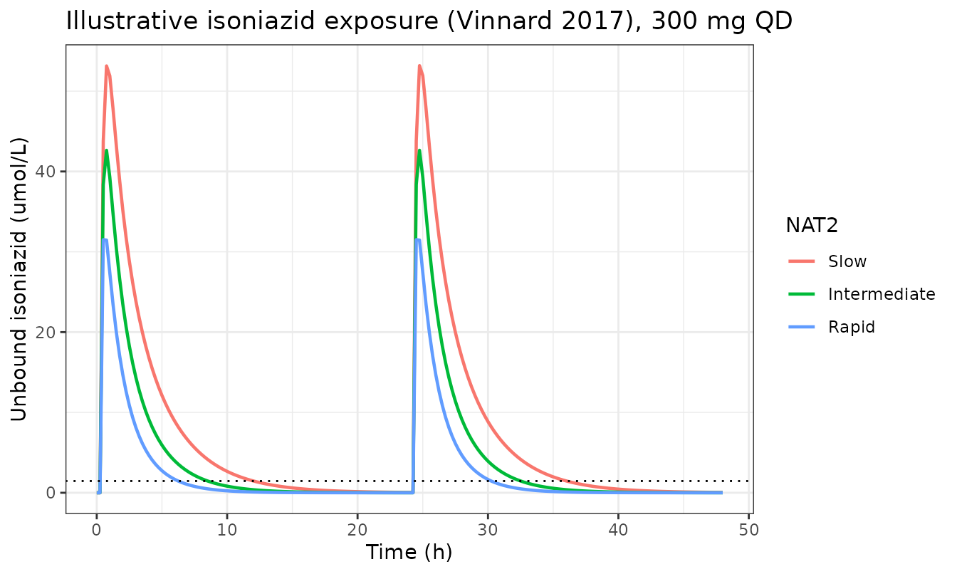
Typical-value unbound isoniazid concentrations by NAT2 phenotype from Vinnard_2017_isoniazid, 300 mg QD, converted to the molar effect-site scale the Cordes 2016 PD model expects.
Feeding each trajectory into the PD model. Note the time-unit change: the PK model runs in hours, the PD model in days.
pd_runs <- lapply(levels(pk_profiles$phenotype), function(ph) {
  prof <- pk_profiles |>
    filter(phenotype == ph) |>
    transmute(time = time / 24, CEFFECT = ceffect) |> # h -> day
    distinct(time, .keep_all = TRUE) |>
    arrange(time)
  s <- rxode2::rxSolve(mod, prof, returnType = "data.frame")
  s$phenotype <- ph
  s
}) |>
  bind_rows() |>
  mutate(phenotype = factor(phenotype, levels = phenotypes$phenotype))

ggplot(pd_runs, aes(time, log10(bact), colour = phenotype)) +
  geom_line(linewidth = 0.8) +
  labs(
    x = "Time (days)", y = "Burden (log10 CFU/L)", colour = "NAT2",
    title = "Illustrative burden over 2 days, 300 mg QD"
  ) +
  theme_bw()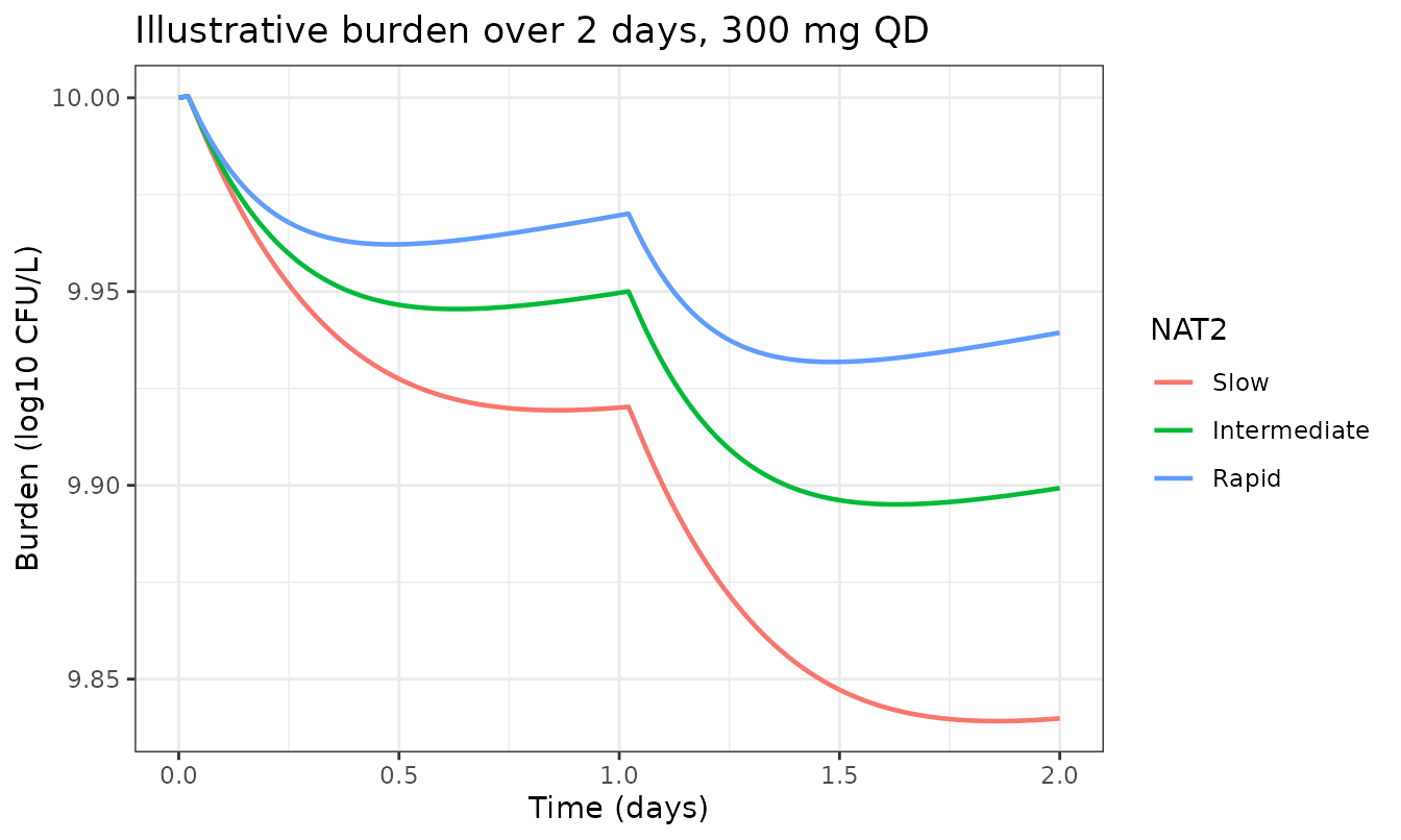
Mycobacterial burden over two days of 300 mg QD isoniazid, driven by the illustrative NAT2-specific exposures above.
eba <- pd_runs |>
  group_by(phenotype) |>
  summarise(
    eba_2day = (log10(first(bact)) - log10(last(bact))) / 2,
    .groups = "drop"
  )

# Fail loudly if a phenotype is missing, so the comparisons below cannot
# silently reduce to a zero-length (vacuously TRUE) test.
eba_of <- function(ph) {
  v <- eba$eba_2day[eba$phenotype == ph]
  if (length(v) != 1L) stop("no unique EBA row for phenotype '", ph, "'")
  v
}
stopifnot(identical(sort(as.character(eba$phenotype)),
                    sort(phenotypes$phenotype)))

# Cordes 2016's central claim: at the standard 300 mg QD dose, EBA falls
# monotonically from slow to intermediate to rapid acetylators.
stopifnot(
  nrow(eba) == 3L,
  eba_of("Slow") > eba_of("Intermediate"),
  eba_of("Intermediate") > eba_of("Rapid"),
  # And all three are genuinely bactericidal on this illustrative exposure.
  all(eba$eba_2day > 0)
)

eba |>
  rename("NAT2 phenotype" = phenotype, "2-day EBA (log10 CFU/day)" = eba_2day) |>
knitr::kable(digits = 4)| NAT2 phenotype | 2-day EBA (log10 CFU/day) |
|---|---|
| Slow | 0.0801 |
| Intermediate | 0.0504 |
| Rapid | 0.0303 |
The ordering slow > intermediate > rapid is Cordes 2016’s headline finding, and it is recovered here from a completely independent PK model. The magnitudes are not the paper’s - they depend on the substituted PK - which is exactly why the assertion above tests the ordering and not the values.
Why these EBA magnitudes are low
The 2-day EBAs above are around 0.03-0.08 log10 CFU/day, well below
the roughly 0.5 log10 CFU/day measured for isoniazid. That gap is a
property of the exposure, not of the PD parameters: the Vinnard
2017 plasma profile spends only a couple of hours per day near the
ec50, and with a Hill coefficient of 0.56 the sigmoid
responds only weakly to short peaks.
Held at a constant concentration in the therapeutic range, the same model produces EBAs much closer to the measured value:
clamped <- tibble::tibble(ceffect = c(10, 20, 36.8, 53, 100, 300)) |>
  rowwise() |>
  mutate(eba = -knet_at(ceffect)) |>
  ungroup()

stopifnot(
  # Monotone in exposure, and bracketing the measured EBA region from below.
  all(diff(clamped$eba) > 0),
  max(clamped$eba) < emax_used # can never exceed Emax
)

clamped |>
  rename("CEFFECT (umol/L)" = ceffect, "EBA (log10 CFU/day)" = eba) |>
knitr::kable(digits = 4)| CEFFECT (umol/L) | EBA (log10 CFU/day) |
|---|---|
| 10.0 | 0.1528 |
| 20.0 | 0.2010 |
| 36.8 | 0.2461 |
| 53.0 | 0.2733 |
| 100.0 | 0.3190 |
| 300.0 | 0.3871 |
Cordes 2016 drove its PD model with PBPK-derived lung
interstitial exposure, which is more sustained than a
plasma-derived proxy, and separately notes that its deliberately
conservative MIC “causes the model to rather underestimate the EBA”.
Both effects push in the same direction as what is seen here. The
alternative Km reading discussed in the Errata is
not the explanation: it raises these EBAs by only 10-20%.
Relative treatment efficacy
Cordes 2016 equation 4 expresses efficacy for each individual relative to the same individual as a slow acetylator on the standard 300 mg QD regimen, which is defined as 100%.
benchmark <- eba_of("Slow")

eba |>
  mutate(relative_efficacy_pct = 100 * eba_2day / benchmark) |>
  select(phenotype, relative_efficacy_pct) |>
  rename("NAT2 phenotype" = phenotype, "Relative efficacy (%)" = relative_efficacy_pct) |>
knitr::kable(digits = 1)| NAT2 phenotype | Relative efficacy (%) |
|---|---|
| Slow | 100.0 |
| Intermediate | 62.9 |
| Rapid | 37.9 |
Cordes 2016 reports 44.2% and 28.2% for immune-deficient intermediate and fast acetylators on this regimen (Results, “Treatment efficacy”). The values here differ because the exposure driving them is Vinnard 2017’s, not the paper’s PBPK - see the caveat above.
Assumptions and deviations
Errata and resolved conflicts in the source
1. The N0 factor printed in equations 1 and 3 is
not applied. Equation 3 reads
dN/dt = N0 * [mu - beta0 - gamma]. Three independent lines
of evidence say the rate balance carries no such multiplier, and the
model file omits it:
- The supplement writes the identical model as equation A1 with no
N0factor at all, and gives every term units of log10 CFU/day. - Only without it does the paper’s own arithmetic close:
mu - beta0 = 0.0428 - 0.0219 = 0.0209log10 CFU/day, exactly the literature-averaged untreated immunocompetent growth rate the supplement reports. WithN0 = 10it would be 0.209. - Only without it is the saturated kill rate the right size for
isoniazid:
Emax = 0.534log10 CFU/day against a measured 2-day EBA of roughly 0.5. WithN0 = 10the model would predict 5.3 log10 CFU/day, an order of magnitude high.
Because dN/dt does not depend on N,
N0 is a pure initial condition, and Table 5 itself
annotates it “Arbitrary”.
2. mu is taken as 0.0428 log10 CFU/day
(supplement), not the 0.048 printed in Table 5. Table 5 is
internally inconsistent: its own beta0 of 0.0219 is exactly
the supplement’s mu_ID (0.0428) - mu_IC (0.0209), and
supplement equation A3 states that identity directly. With
mu = 0.048 the untreated immunocompetent growth rate would
be 0.0261 rather than the literature-derived 0.0209. This is gated by an
assertion in the “Untreated growth” section above. A reader wanting
Table 5 as printed can override with
rxode2::rxSolve(mod, ..., params = c(lkgrowth = log(0.048))).
Note also that supplement equation A2 does not reproduce its own
stated result: 0.0209 * 0.295 / 0.1355 = 0.0455, not the
0.0428 the supplement reports. The 0.0428 value is retained because it
is the one that satisfies A3 and matches Table 5’s beta0;
the A2 discrepancy is most likely rounding in the reported murine growth
rates.
3. Km is carried as a dimensionless multiple of
the MIC, not as a concentration in umol/L. Equation 2 reads
Emax*(C/MIC)^h / (Km^h + (C/MIC)^h). The right-hand
denominator term is dimensionless, so Km must be
dimensionless too, placing the half-maximal effect at
C = 25.19 * MIC = 36.8 umol/L. Table 5 instead annotates
Km as “umol/liter”, and the accompanying prose calls it
“the INH concentration at which half the maximal antimicrobial effect is
reached”, which would place the half-effect at 25.19 umol/L and require
equation 2’s denominator to have been (Km/MIC)^h.
The equation is followed here for two reasons: it is the only reading
under which the printed equation is dimensionally valid as written, and
the C/MIC normalisation is inherited from Czock &
Keller 2007 (reference 47), whose antimicrobial sigmoid is written in
MIC multiples. The two readings differ by a factor of MIC = 1.46 in the
half-effect concentration. The paper reports no absolute lung
concentration against which they could be discriminated, because the
concentrations that would settle it come from the unported PBPK layer. A
reader preferring the Table 5 reading can override with
params = c(lec50 = log(25.19 / 1.46)).
Scope and substitutions
-
The PBPK layer is not ported. Reasons are given in
full in the first section. No INH PK is implied by this file;
CEFFECTmust be supplied. - The chaining section substitutes Vinnard 2017 PK. This is an illustration of how to use the model and a test of the paper’s qualitative acetylator ordering. It is not a replication of Cordes 2016’s numbers, and the assertions in that section test ordering and sign only.
- Plasma-to-effect-site conversion. The chaining section multiplies plasma concentration by the fraction unbound (0.90, Cordes 2016 Table 1) and converts to molar units with MW 137.14 g/mol (Table 1). Treating unbound plasma as a proxy for the lung interstitium follows the paper’s own Discussion, but within Cordes 2016 the interstitial concentration is a PBPK output, not this ratio.
-
No variability and no residual error. Cordes 2016
reports neither for the PD layer (goodness of fit is given only as
R^2 = 0.6, P < 0.001), so there are no eta terms andaddSdis fixed at 0. The model is for deterministic typical-value simulation. - Metabolite toxicity is not represented. The paper’s toxicity index is the AUC of hydrazine and acetylhydrazine in the intracellular liver space - an output of the unported PBPK layer, with no separate PD model attached to it. There is no equation in the paper that could be carried here independently of the platform model.
- The 2-day horizon is the paper’s. Cordes 2016 states that treatment durations of months could not be analysed for lack of adequate data, and that resistant subpopulations were not modelled. The model should not be extrapolated to long-course therapy.
-
The MIC is conservative by design. Cordes 2016
chose 0.2 mg/L to cover most susceptible strains, noting that most fall
between 0.05 and 0.1 mg/L, and that this “causes the model to rather
underestimate the EBA”. Change the
micparameter to apply the model to a specific isolate.