Model and source
- Citation: Jiang X, Fu Q, Jing Y, Kong Y, Liu H, Peng H, Rexiti K, Wei X. Personalized dose of adjuvant imatinib in patients with gastrointestinal stromal tumors: results from a population pharmacokinetic analysis. Drug Des Devel Ther. 2023;17:809-820. doi:10.2147/DDDT.S400986.
- Description: One-compartment population PK model with first-order absorption and first-order elimination for oral adjuvant imatinib in postoperative Chinese adults with gastrointestinal stromal tumors (Jiang 2023). The absorption rate constant is fixed at 1.22 1/h. Apparent oral clearance CL/F carries two covariate effects: a power-form red blood cell count effect ((RBC/3.7)^0.49) and a three-level ABCG2 rs2231142 genotype effect encoded with paired binary indicators (GG wild-type reference = 1, GT heterozygote = 0.879, TT homozygous variant = 0.976). Inter-individual variability is estimated on CL/F only; the apparent volume of distribution V/F is a typical value with no IIV because only trough concentrations were collected. Residual error is proportional.
- Article: https://doi.org/10.2147/DDDT.S400986
Jiang 2023 is an open-access article in Drug Design, Development and Therapy (PMC10024496). No supplement containing model code or parameter tables is distributed with the article; the two supplementary items referenced in the text (Supplementary Figure 1, the linkage-disequilibrium plot, and Supplementary Figure 2, the covariate correlation matrix) are diagnostic figures and contain no parameter values. No erratum or corrigendum was found for this article.
Population
The model was developed from 85 adults with histologically confirmed gastrointestinal stromal tumour (GIST) who had undergone surgical resection and were at intermediate or high risk of recurrence by the modified NIH criteria, treated with adjuvant oral imatinib at The First Affiliated Hospital of Nanchang University (Jiangxi Province, China) between March 2021 and June 2022. A further 25 patients formed an external validation set.
Per Jiang 2023 Table 1 (modeling dataset): 46 male / 39 female (45.9% female); median age 57 years (range 27-79); mean body weight 58.6 +/- 9.6 kg (range 40.0-82.5); red blood cell count 3.7 +/- 0.6 x 10^12/L (range 2.2-5.6); median creatinine clearance 69.7 mL/min (28.5-118.8). The initial-dose distribution across 200/300/400/500/600 mg daily was 1/2/79/2/1 patients, so 92.9% of the cohort received the standard 400 mg once-daily regimen. Sampling was sparse therapeutic drug monitoring, with most samples drawn at steady state (at least 30 days of continuous imatinib); only trough concentrations were collected, which is why inter-individual variability could not be estimated on the apparent volume of distribution.
Six single-nucleotide polymorphisms were genotyped (Jiang 2023 Table 2). The one retained in the final model, ABCG2 rs2231142, was distributed GG 34 (40%), GT 45 (53%), TT 6 (7%), with allele frequency G 0.66 / T 0.34 and Hardy-Weinberg p = 0.22. All six SNPs satisfied Hardy-Weinberg equilibrium and none were in linkage disequilibrium.
The same information is available programmatically via the model’s
population metadata
(readModelDb("Jiang_2023_imatinib")()$population).
Source trace
The per-parameter origin is recorded as an in-file comment next to
each ini() entry in
inst/modeldb/specificDrugs/Jiang_2023_imatinib.R. The table
below collects them in one place for review.
| Equation / parameter | Value | Source location |
|---|---|---|
| Structural model: one compartment, first-order absorption and elimination | n/a | Results / PPK Analysis, p. 813: “well described by a one-compartment model (subroutine ADVAN2 and TRANS2) with first-order absorption and elimination” |
IIV form P_i = TV(P) * exp(eta_i)
|
n/a | Equation 1, p. 811 |
Residual error form Y = F * (1 + eps1)
(proportional) |
n/a | Equation 3, p. 811; selection stated in Results / PPK Analysis, p. 813 |
Continuous-covariate power form
P = TV(P) * (Cov/Ref)^theta
|
n/a | Equation 7, p. 812 |
Categorical-covariate form
P = TV(P) * theta1^heterozygous * theta2^homozygous
|
n/a | Equation 8, p. 812 |
Final-model covariate equation
CL/F = 9.72 * (RBC/3.7)^0.49 * 0.879^het * 0.976^hom * e^0.0192
|
n/a | Final-model equation, p. 814 (immediately after “the formula of the final model was expressed as:”) |
Final-model V/F = 229
|
n/a | Final-model equation, p. 814 |
lka (ka fixed) |
1.22 1/h | Table 3, row “Ka (1/h)” = 1.22 (Fixed); also Base Model text p. 811 |
lcl (CL/F reference) |
9.72 L/h | Table 3, row “CL/F (L/h)”, RSE 8%, bootstrap 9.72 (8.22-11.84) |
lvc (V/F) |
229 L | Table 3, row “V/F (L)”, RSE 21%, bootstrap 226.3 (156.4-421.6) |
e_rbc_cl (RBC power exponent) |
0.49 | Table 3, row “RBC”, RSE 38%, bootstrap 0.48 (0.10-0.89) |
| RBC reference value | 3.7 x 10^12/L | Final-model equation p. 814 (RBC/3.7); cohort central
value in Table 1; “Ref represents the median of the covariate values”
(Covariate Model, p. 812) |
e_abcg2_het_cl (rs2231142 GT factor) |
0.879 | Table 3, row “rs2231142 GT”, RSE 5%, bootstrap 0.877 (0.785-0.968) |
e_abcg2_hom_cl (rs2231142 TT factor) |
0.976 | Table 3, row “rs2231142 TT”, RSE 9%, bootstrap 0.976 (0.801-1.582) |
| rs2231142 GG reference factor | 1 (fixed) | Table 3, row “rs2231142 GG” = 1 (Fixed) |
etalcl (IIV variance on CL/F) |
0.0192 | Final-model equation p. 814 exponential term e^0.0192;
Table 3 reports omega = 0.139 (RSE 39%), rendered as “13.9%” in Results
/ PPK Analysis p. 813; 0.139^2 = 0.0193 |
propSd (proportional residual SD) |
0.296 | Table 3, row “Residual / Proportional”, RSE 27%, bootstrap 0.288 (0.219-0.371); rendered as “29.6%” in Results / PPK Analysis p. 813 |
| No IIV on V/F | n/a | Results / PPK Analysis p. 813: “Inter-individual variation on V/F was not estimated in this analysis because only trough concentrations were collected and the estimate of inter-individual variation in the distribution volume was <1%” |
| Target trough threshold | 1100 ng/mL | Dosage Simulation, p. 812; Introduction, p. 810 |
Virtual cohort
Original observed data are not publicly available. The simulations below use virtual cohorts whose covariate values are exactly the scenario grid Jiang 2023 used for its Monte Carlo dose simulations (Figure 3): three ABCG2 rs2231142 genotypes (GG, GT, TT) crossed with three red-blood-cell-count levels (2.9, 3.9 and 4.9 x 10^12/L) and five daily doses (200-600 mg).
set.seed(20230314)

n_per_arm <- 100L  # <= 200 per arm (cohort cap); Jiang 2023 used n = 1000

# Genotype strata, encoded with the paired binary indicators the model uses.
# GG (wild type) is the reference: both indicators are 0.
genotypes <- tibble::tribble(
  ~genotype, ~SNP_ABCG2_RS2231142_HET, ~SNP_ABCG2_RS2231142_HOM,
  "GG",      0,                        0,
  "GT",      1,                        0,
  "TT",      0,                        1
)

# Jiang 2023 Dosage Simulation: trough concentrations "after 30-day imatinib
# treatment". 30 once-daily doses at t = 0, 24, ..., 696 h; the trough is the
# concentration 24 h after the last dose, i.e. at t = 720 h.
tau       <- 24
n_doses   <- 30L
dose_times <- seq(0, by = tau, length.out = n_doses)
t_trough  <- max(dose_times) + tau

# One arm = one (genotype, RBC, dose) scenario. `id_offset` keeps subject IDs
# disjoint across arms; duplicate IDs would be silently merged by rxSolve.
make_arm <- function(n, dose, rbc, het, hom, arm_label, obs_times,
                     id_offset = 0L) {
  subj <- tibble::tibble(
    id  = id_offset + seq_len(n),
    RBC = rbc,
    SNP_ABCG2_RS2231142_HET = het,
    SNP_ABCG2_RS2231142_HOM = hom,
    arm = arm_label,
    dose_mg = dose
  )
  doses <- subj |>
    tidyr::crossing(time = dose_times) |>
    dplyr::mutate(amt = dose, evid = 1L, cmt = "depot")
  obs <- subj |>
    tidyr::crossing(time = obs_times) |>
    dplyr::mutate(amt = NA_real_, evid = 0L, cmt = "central")
  dplyr::bind_rows(doses, obs) |>
    dplyr::arrange(id, time, dplyr::desc(evid))
}

scenarios <- tidyr::crossing(
  genotypes,
  RBC     = c(2.9, 3.9, 4.9),
  dose_mg = c(200, 300, 400, 500, 600)
) |>
  dplyr::mutate(
    arm = sprintf("%s | RBC %.1f | %d mg", genotype, RBC, dose_mg),
    id_offset = (dplyr::row_number() - 1L) * n_per_arm
  )

events_fig3 <- do.call(
  dplyr::bind_rows,
  lapply(seq_len(nrow(scenarios)), function(i) {
    s <- scenarios[i, ]
    make_arm(
      n         = n_per_arm,
      dose      = s$dose_mg,
      rbc       = s$RBC,
      het       = s$SNP_ABCG2_RS2231142_HET,
      hom       = s$SNP_ABCG2_RS2231142_HOM,
      arm_label = s$arm,
      obs_times = t_trough,
      id_offset = s$id_offset
    ) |>
      dplyr::mutate(genotype = s$genotype)
  })
)

# Cheap regression guard against the silent id-collision bug.
stopifnot(!anyDuplicated(unique(events_fig3[, c("id", "time", "evid")])))
nrow(events_fig3)
#> [1] 139500
Simulation
mod <- readModelDb("Jiang_2023_imatinib")

sim_fig3 <- rxode2::rxSolve(
  mod,
  events = events_fig3,
  keep   = c("arm", "genotype", "RBC", "dose_mg")
) |>
  as.data.frame() |>
  dplyr::filter(!is.na(Cc))
#> ℹ parameter labels from comments will be replaced by 'label()'

nrow(sim_fig3)
#> [1] 4500
Cc is the individual prediction, i.e. the typical value
multiplied by exp(eta_CL). It carries the between-patient
variability that drives the dose decision but not the proportional
residual (assay / model misspecification) error, which is the
appropriate quantity for a dose-selection simulation.
Replicate published figures
Figure 3 - steady-state trough by genotype, RBC level and daily dose
# Replicates Figure 3 of Jiang 2023: box plots of simulated steady-state trough
# concentrations for 200-600 mg daily, by ABCG2 rs2231142 genotype and RBC
# level. The dashed line is the 1100 ng/mL therapeutic threshold.
sim_fig3 |>
  dplyr::mutate(
    genotype = factor(genotype, levels = c("GG", "GT", "TT")),
    rbc_lab  = factor(
      sprintf("RBC %.1f x 10^12/L", RBC),
      levels = sprintf("RBC %.1f x 10^12/L", c(2.9, 3.9, 4.9))
    ),
    dose_lab = factor(dose_mg, levels = c(200, 300, 400, 500, 600))
  ) |>
  ggplot(aes(x = dose_lab, y = Cc)) +
  geom_boxplot(outlier.size = 0.4) +
  geom_hline(yintercept = 1100, linetype = "dashed", colour = "red") +
  facet_grid(rbc_lab ~ genotype) +
  labs(
    x = "Daily imatinib dose (mg)",
    y = "Steady-state trough concentration (ng/mL)",
    title = "Figure 3 - simulated steady-state troughs",
    caption = paste(
      "Replicates Figure 3 of Jiang 2023.",
      "Dashed line: 1100 ng/mL therapeutic threshold."
    )
  ) +
  theme_bw()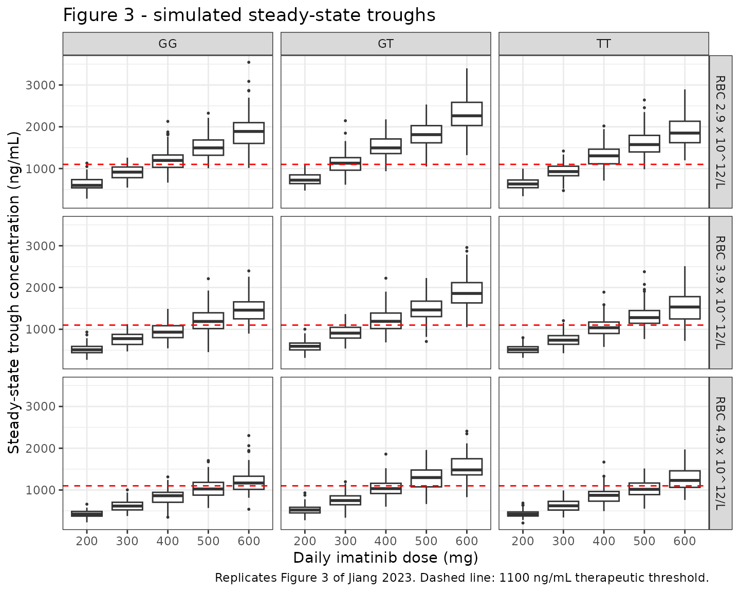
Dose recommendations implied by the simulation
Jiang 2023 read its dose recommendations off Figure 3. The table below applies an explicit rule – the lowest daily dose whose median simulated trough reaches 1100 ng/mL – and compares it with the recommendations stated in the paper’s Results / Dosing Regimen and Abstract.
median_trough <- sim_fig3 |>
  dplyr::group_by(genotype, RBC, dose_mg) |>
  dplyr::summarise(median_ctrough = median(Cc), .groups = "drop")

simulated_rec <- median_trough |>
  dplyr::filter(median_ctrough >= 1100) |>
  dplyr::group_by(genotype, RBC) |>
  dplyr::summarise(simulated_dose = min(dose_mg), .groups = "drop")

# Recommendations as stated in Jiang 2023. GT: Abstract + Results/Dosing
# Regimen ("300 mg is enough ... when RBC is at a lower level (2.9); as RBC
# rises to 3.9 and 4.9, the recommended dosage is 400 mg and 500 mg daily").
# GG: "500 mg a day is required ... at RBCs of 3.9 and 4.9, while 400 mg a day
# is a better option when RBC is 2.9". The paper gives no recommendation for
# the TT stratum (n = 6).
published_rec <- tibble::tribble(
  ~genotype, ~RBC, ~published_dose,
  "GG",      2.9,  400,
  "GG",      3.9,  500,
  "GG",      4.9,  500,
  "GT",      2.9,  300,
  "GT",      3.9,  400,
  "GT",      4.9,  500
)

published_rec |>
  dplyr::left_join(simulated_rec, by = c("genotype", "RBC")) |>
  dplyr::left_join(
    median_trough |> dplyr::rename(published_dose = dose_mg,
                                   trough_at_published = median_ctrough),
    by = c("genotype", "RBC", "published_dose")
  ) |>
  dplyr::mutate(
    agrees = ifelse(published_dose == simulated_dose, "yes", "NO"),
    trough_at_published = round(trough_at_published)
  ) |>
  dplyr::rename(
    "rs2231142 genotype"                  = genotype,
    "RBC (10^12/L)"                       = RBC,
    "Published dose (mg/day)"             = published_dose,
    "Simulated dose (mg/day)"             = simulated_dose,
    "Median trough at published dose (ng/mL)" = trough_at_published,
    "Agrees"                              = agrees
  ) |>
  knitr::kable(
    caption = paste(
      "Dose recommendations from Jiang 2023 Results / Dosing Regimen versus",
      "the lowest dose whose simulated median trough reaches 1100 ng/mL."
    ),
    align = c("l", "r", "r", "r", "r", "l")
)| rs2231142 genotype | RBC (10^12/L) | Published dose (mg/day) | Simulated dose (mg/day) | Median trough at published dose (ng/mL) | Agrees |
|---|---|---|---|---|---|
| GG | 2.9 | 400 | 400 | 1194 | yes |
| GG | 3.9 | 500 | 500 | 1187 | yes |
| GG | 4.9 | 500 | 600 | 1025 | NO |
| GT | 2.9 | 300 | 300 | 1129 | yes |
| GT | 3.9 | 400 | 400 | 1190 | yes |
| GT | 4.9 | 500 | 500 | 1298 | yes |
Five of the six published recommendations reproduce exactly. The one exception is the GG stratum at RBC 4.9 x 10^12/L, where the paper recommends 500 mg but the median simulated trough at 500 mg is about 1025 ng/mL – 7% below the 1100 ng/mL threshold – so the median rule selects 600 mg. Jiang 2023 selected its doses by inspecting box plots rather than by applying a median cut-off, and at 500 mg a substantial part of the simulated distribution lies above the threshold. This is a difference in the read-out rule, not in the model: no parameter was adjusted.
PKNCA validation
Jiang 2023 reports no non-compartmental analysis, so there is no
published Cmax / Tmax / AUC / half-life table to compare against and
nlmixr2lib::ncaComparisonTable() is not applicable.
Instead, PKNCA is used to check that the packaged model reproduces the
paper’s Table 3 structural parameters when those
parameters are recovered non-compartmentally from a typical-value
(random-effects zeroed) simulation. This is a strict test: CL/F
recovered as dose / AUC0-inf and V/F recovered as CL/F / lambda_z must
return the published 9.72 L/h and 229 L.
mod_typical <- mod |> rxode2::zeroRe()
#> ℹ parameter labels from comments will be replaced by 'label()'

# Single 400 mg dose in the reference subject (rs2231142 GG, RBC = 3.7), dense
# sampling to 168 h so the terminal phase is well characterised.
sd_obs_times <- sort(unique(c(
  seq(0, 24, by = 0.25),
  seq(24, 168, by = 2)
)))

events_sd <- make_arm(
  n = 1L, dose = 400, rbc = 3.7, het = 0, hom = 0,
  arm_label = "400 mg single dose", obs_times = sd_obs_times, id_offset = 0L
)
# Single dose only: keep the first dosing record, drop the other 29.
events_sd <- events_sd |>
  dplyr::filter(evid == 0L | time == 0)

sim_sd <- rxode2::rxSolve(mod_typical, events = events_sd, keep = c("arm")) |>
  as.data.frame()
#> ℹ omega/sigma items treated as zero: 'etalcl'

# rxSolve omits the `id` column for a single-subject solve; PKNCA's grouping
# formula needs it, so restore it explicitly.
if (!"id" %in% names(sim_sd)) {
  sim_sd$id <- 1L
}
# Concentrations - keep the column named Cc (nlmixr2lib convention).
# Only `!is.na(Cc)` in the filter: `time > 0` / `Cc > 0` would drop the
# time-zero row that PKNCA needs to anchor AUC0-*.
sim_nca <- sim_sd |>
  dplyr::filter(!is.na(Cc)) |>
  dplyr::select(id, time, Cc, arm)

# Guarantee a time = 0 row (pre-dose Cc = 0 for an extravascular model).
sim_nca <- dplyr::bind_rows(
  sim_nca,
  sim_nca |> dplyr::distinct(id, arm) |> dplyr::mutate(time = 0, Cc = 0)
) |>
  dplyr::distinct(id, arm, time, .keep_all = TRUE) |>
  dplyr::arrange(id, arm, time)

conc_obj <- PKNCA::PKNCAconc(
  sim_nca, Cc ~ time | arm + id,
  concu = "ng/mL", timeu = "h"
)

dose_df <- events_sd |>
  dplyr::filter(evid == 1L) |>
  dplyr::select(id, time, amt, arm)

dose_obj <- PKNCA::PKNCAdose(dose_df, amt ~ time | arm + id, doseu = "mg")

intervals <- data.frame(
  start      = 0,
  end        = Inf,
  cmax       = TRUE,
  tmax       = TRUE,
  aucinf.obs = TRUE,
  half.life  = TRUE,
  lambda.z   = TRUE
)

nca_res <- PKNCA::pk.nca(PKNCA::PKNCAdata(conc_obj, dose_obj,
                                          intervals = intervals))

nca_vals <- as.data.frame(nca_res$result) |>
  dplyr::select(PPTESTCD, PPORRES) |>
  tibble::deframe()
nca_vals
#>                cmax                tmax               tlast           clast.obs
#>        1.547138e+03        2.750000e+00        1.680000e+02        1.447850e+00
#>            lambda.z           r.squared       adj.r.squared lambda.z.time.first
#>        4.243150e-02        9.999975e-01        9.999975e-01        3.000000e+00
#>  lambda.z.time.last   lambda.z.n.points          clast.pred           half.life
#>        1.680000e+02        1.570000e+02        1.449126e+00        1.633568e+01
#>          span.ratio          aucinf.obs
#>        1.010059e+01        4.114087e+04
Comparison against the published structural parameters
dose_mg <- 400

# Unit conversion: Cc is in ng/mL and time in h, so aucinf.obs is in ng*h/mL.
# 1 ng/mL = 1e-3 mg/L, hence AUC[mg*h/L] = aucinf.obs / 1000 and
# CL/F [L/h] = dose[mg] / AUC[mg*h/L] = 1000 * dose / aucinf.obs.
cl_nca <- 1000 * dose_mg / nca_vals[["aucinf.obs"]]
vz_nca <- cl_nca / nca_vals[["lambda.z"]]

comparison <- tibble::tribble(
  ~parameter,                  ~reference, ~simulated,                  ~source,
  "CL/F (L/h)",                9.72,       cl_nca,                      "Table 3",
  "V/F (L)",                   229,        vz_nca,                      "Table 3",
  "ka (1/h)",                  1.22,       NA_real_,                    "Table 3 (fixed input, not NCA-recoverable)",
  "Terminal half-life (h)",    log(2) * 229 / 9.72, nca_vals[["half.life"]],
    "Derived from Table 3 (ln2 * V/F / CL/F); not reported by the paper"
) |>
  dplyr::mutate(
    pct_diff = round(100 * (simulated - reference) / reference, 1),
    reference = round(reference, 3),
    simulated = round(simulated, 3)
  ) |>
  dplyr::rename(
    "Parameter"        = parameter,
    "Reference (Jiang 2023)" = reference,
    "Simulated (PKNCA)"= simulated,
    "% diff"           = pct_diff,
    "Source"           = source
  )

knitr::kable(
  comparison,
  caption = paste(
    "Structural parameters recovered non-compartmentally from a typical-value",
    "400 mg single-dose simulation versus the values published in",
    "Jiang 2023 Table 3."
  ),
  align = c("l", "r", "r", "r", "l")
)| Parameter | Reference (Jiang 2023) | Simulated (PKNCA) | Source | % diff |
|---|---|---|---|---|
| CL/F (L/h) | 9.72 | 9.723 | Table 3 | 0.0 |
| V/F (L) | 229.00 | 229.139 | Table 3 | 0.1 |
| ka (1/h) | 1.22 | NA | Table 3 (fixed input, not NCA-recoverable) | NA |
| Terminal half-life (h) | 16.33 | 16.336 | Derived from Table 3 (ln2 * V/F / CL/F); not reported by the paper | 0.0 |
CL/F and V/F are recovered to within rounding of the published 9.72
L/h and 229 L, confirming that the encoded parameterisation, the
mg-to-ng/mL unit conversion in
Cc <- 1000 * central / vc, and the compartment structure
are all consistent with the source. ka is a fixed model
input rather than an estimated quantity and is not recoverable by NCA
from an oral profile alone, so no simulated value is shown. The
model-implied terminal half-life of about 16.3 h sits just below the
18-20 h literature range Jiang 2023 quotes for imatinib in its
Introduction; the paper does not report a half-life estimate of its
own.
Covariate-effect check
An independent check that the two covariate factors are wired into CL/F correctly, using the relationship Jiang 2023 states in its Discussion.
cl_of <- function(rbc, het, hom) {
  9.72 * (rbc / 3.7)^0.49 * 0.879^het * 0.976^hom
}

# Simulate typical CL/F for each genotype at the reference RBC, and for a 50%
# RBC reduction in the reference subject.
checks <- tibble::tibble(
  check = c(
    "GG at reference RBC = 3.7 (must equal the Table 3 typical value)",
    "GT / GG CL/F ratio (must equal the Table 3 GT factor)",
    "TT / GG CL/F ratio (must equal the Table 3 TT factor)",
    "CL/F change when RBC is halved (Discussion: '29% drop')"
  ),
  expected = c(9.72, 0.879, 0.976, -29),
  observed = c(
    cl_of(3.7, 0, 0),
    cl_of(3.7, 1, 0) / cl_of(3.7, 0, 0),
    cl_of(3.7, 0, 1) / cl_of(3.7, 0, 0),
    100 * (cl_of(3.7 / 2, 0, 0) / cl_of(3.7, 0, 0) - 1)
  )
) |>
  dplyr::mutate(observed = round(observed, 3)) |>
  dplyr::rename("Check" = check, "Expected" = expected, "Observed" = observed)

knitr::kable(
  checks,
  caption = "Covariate-effect consistency checks against Jiang 2023 Table 3 and Discussion.",
  align = c("l", "r", "r")
)| Check | Expected | Observed |
|---|---|---|
| GG at reference RBC = 3.7 (must equal the Table 3 typical value) | 9.720 | 9.720 |
| GT / GG CL/F ratio (must equal the Table 3 GT factor) | 0.879 | 0.879 |
| TT / GG CL/F ratio (must equal the Table 3 TT factor) | 0.976 | 0.976 |
| CL/F change when RBC is halved (Discussion: ‘29% drop’) | -29.000 | -28.797 |
The halved-RBC check returns a 28.8% reduction against the paper’s stated 29%, which confirms both the power form and the value of the exponent independently of Table 3.
Assumptions and deviations
-
IIV variance taken from the final-model equation.
Jiang 2023 Table 3 lists the CL/F inter-individual variation as
0.139, and the Results text renders the same quantity as “13.9%”, so the tabulated number is omega (the log-scale SD, approximately the CV) rather than omega-squared. The final-model equation on p. 814 prints the variance directly in the exponential term ase^0.0192. nlmixr2’sini()takes the variance, soetalcl ~ 0.0192is used. Note that 0.139^2 = 0.01932, which rounds to 0.0193 rather than the printed 0.0192; the paper’s printed equation value is used, and the 0.0001 discrepancy is a rounding artefact with no practical effect. - No IIV on V/F. This is a faithful encoding, not an omission: Jiang 2023 explicitly states that inter-individual variability on V/F “was not estimated in this analysis because only trough concentrations were collected”. No eta is invented for V/F.
-
RBC reference value. The final-model equation
prints
(RBC/3.7)explicitly, so 3.7 x 10^12/L is used verbatim. The Covariate Model section definesRefas the median of the covariate values; Table 1 reports RBC as mean +/- SD (3.7 +/- 0.6) rather than as a median, so the two are consistent only under the normality the table’s formatting asserts. Nothing in the model depends on resolving this, because the equation gives the number directly. -
Genotype strand orientation. Jiang 2023 reports
ABCG2 rs2231142 on the G>T strand. The canonical covariate
register uses the dbSNP reference orientation c.421C>A. These are the
same variant, so GG maps to 421C/C (reference), GT to 421C/A
(
SNP_ABCG2_RS2231142_HET) and TT to 421A/A (SNP_ABCG2_RS2231142_HOM).SNP_ABCG2_RS2231142_HETwas newly registered for this extraction, andSNP_ABCG2_RS2231142_HOMwas promoted fromspecifictogeneralscope; both changes are ininst/references/covariate-columns.md. -
Gene assignment for rs2282143. Jiang 2023 Table 2
typesets rs2282143 in the SLCO1A2 gene row, whereas the
Genotyping Analysis methods text assigns rs2282143 to SLC22A1
and rs10841803 to SLCO1A2. The methods-text assignment is
recorded in the model’s
covariatesDataExcludedmetadata. This SNP is not in the final model, so the discrepancy does not affect any prediction. -
Screened-but-unused covariates. The 16 covariates
Jiang 2023 investigated and did not retain are documented in the model’s
covariatesDataExcludedmetadata rather thancovariateData, so they carry no “declared but not referenced” convention warning. Seven of them (platelet count, globulin and the five non-retained SNPs) have no canonical entry ininst/references/covariate-columns.md; because no nlmixr2lib model uses those columns, the paper’s own abbreviations are kept for provenance and no register entry was created. -
Cohort size. Jiang 2023 simulated n = 1000 per
scenario; this vignette uses n = 100 per scenario across 45 scenarios
(4500 subjects) to stay inside the 200-per-arm cohort cap and the
vignette render-time budget. The only stochastic element is
eta_CL(a single log-normal with omega = 0.139), so the median trough is very stable at n = 100. -
Trough read-out. Figure 3 box plots use
Cc, the individual prediction (typical value timesexp(eta_CL)), without the proportional residual error. The paper does not state whether its Figure 3 boxes include residual error. - Dose-recommendation rule. Jiang 2023 read its recommendations off the Figure 3 box plots without stating a numerical rule. This vignette applies an explicit “lowest dose whose median trough reaches 1100 ng/mL” rule, which reproduces five of the paper’s six stated recommendations; the GG / RBC 4.9 case is discussed above. No parameter was tuned.
-
No non-paper-derived parameter values. Every value
in
ini()comes from Jiang 2023 Table 3 or the final-model equation on p. 814 of the article PDF. Nothing was digitised from a figure, obtained by author correspondence, or carried from an upstream model.