Aripiprazole lauroxil (Hard 2017)
Source:vignettes/articles/Hard_2017_aripiprazole_lauroxil.Rmd
Hard_2017_aripiprazole_lauroxil.RmdModel and source
ui <- rxode2::rxode(readModelDb("Hard_2017_aripiprazole_lauroxil"))
#> ℹ parameter labels from comments will be replaced by 'label()'
#> Warning: some etas defaulted to non-mu referenced, possible parsing error: etaiov_d1_1, etaiov_d1_2, etaiov_d1_3, etaiov_d1_4, etaiov_d1_5, etaiov_d1_6, etaiov_d1_7
#> as a work-around try putting the mu-referenced expression on a simple line- Citation: Hard ML, Mills RJ, Sadler BM, Wehr AY, Weiden PJ, von Moltke L (2017). Pharmacokinetic Profile of a 2-Month Dose Regimen of Aripiprazole Lauroxil: A Phase I Study and a Population Pharmacokinetic Model. CNS Drugs 31(7):617-624. doi:10.1007/s40263-017-0447-7. Parameter estimates from Supplemental Table 7 of the Electronic Supplementary Material. Vp/F, Q/F and the 70 kg weight-centering constant are carried from the earlier aripiprazole lauroxil PopPK model of Hard ML, Mills RJ, Sadler BM, Turncliff RZ, Citrome L (2017) J Clin Psychopharmacol 37(3):289-295, doi:10.1097/JCP.0000000000000691 (not currently in nlmixr2lib).
- Description: Two-compartment population PK model (2MPopPK) for aripiprazole released from the long-acting intramuscular prodrug aripiprazole lauroxil, with lagged zero-order IM input and a first-order oral aripiprazole route, in adults with schizophrenia
- Article: https://doi.org/10.1007/s40263-017-0447-7
- Electronic Supplementary Material (parameter table): https://doi.org/10.1007/s40263-017-0447-7 (Supplementary
file 1,
40263_2017_447_MOESM1_ESM.pdf) - Earlier PopPK model from which Vp/F, Q/F and the weight centering are carried: https://doi.org/10.1097/JCP.0000000000000691
Aripiprazole lauroxil (AL) is an intramuscular extended-release prodrug of aripiprazole. The prodrug itself is not measurable in plasma; the model therefore describes aripiprazole only, entering the systemic circulation as a lagged zero-order input whose duration (43.5 days) exceeds every approved dosing interval. The paper calls this model the 2MPopPK model.
Structure
Supplemental Fig. 1 of the ESM draws seven intramuscular depots and
one oral depot all feeding a single aripiprazole central compartment,
which exchanges with one peripheral compartment and is cleared by CL/F.
The seven IM depots are a NONMEM book-keeping device – the figure’s own
footnote says “a new IM depot was added for each injection … to
accommodate the maximum number of AL injections in the clinical studies
(seven in study A105)” – and the model carries no rate constant
out of an IM depot. Each depot contributes a zero-order input
of duration D1 beginning ALAG after the
injection, so the seven depots superpose exactly onto a single lagged
modelled-duration input to central. That is how the model
is encoded here, which also removes the artificial seven-injection
ceiling.
cat(paste(rxode2::modelExtract(ui), collapse = "\n"))
#> oc1 <- (OCC == 1)
#> oc2 <- (OCC == 2)
#> oc3 <- (OCC == 3)
#> oc4 <- (OCC == 4)
#> oc5 <- (OCC == 5)
#> oc6 <- (OCC == 6)
#> oc7 <- (OCC == 7)
#> iov_d1 <- oc1 * etaiov_d1_1 + oc2 * etaiov_d1_2 + oc3 * etaiov_d1_3 + oc4 * etaiov_d1_4 + oc5 * etaiov_d1_5 + oc6 * etaiov_d1_6 + oc7 * etaiov_d1_7
#> ka <- exp(lka + etalka)
#> cl <- exp(lcl + etalcl) * e_cyp2d6_pm_cl^CYP2D6_PM
#> vc <- exp(lvc + etalvc) * (WT/70)^e_wt_vc
#> vp <- exp(lvp + etalvp)
#> q <- exp(lq + etalq)
#> d1 <- exp(ld1 + etald1 + iov_d1)
#> tlag <- exp(ltlag + etaltlag)
#> c0 <- exp(lc0 + etalc0)
#> fdepot <- exp(lfdepot)
#> fdepot_im <- exp(lfdepot_im + etalfdepot_im)
#> kel <- cl/vc
#> k12 <- q/vc
#> k21 <- q/vp
#> d/dt(depot) <- -ka * depot
#> d/dt(central) <- ka * depot - kel * central - k12 * central + k21 * peripheral1
#> d/dt(peripheral1) <- k12 * central - k21 * peripheral1
#> central(0) <- c0 * vc/1000
#> f(depot) <- fdepot
#> f(central) <- fdepot_im
#> dur(central) <- d1
#> alag(central) <- tlag
#> Cc <- 1000 * central/vc
#> propSdStudy <- propSdStdyA105 * STUDY_A105 + propSdStdyPrior * (1 - STUDY_A105)
Consequences for a user’s data set:
-
IM aripiprazole lauroxil doses use
cmt = "central"withrate = -2(so rxode2 uses the modelled durationdur(central) <- d1) and the aripiprazole-equivalent dose in mg, not the AL dose. The paper’s mapping is 441 / 662 / 882 / 1064 mg AL = 300 / 450 / 600 / 724 mg aripiprazole equivalent (Sect. 2.2). Withoutrate = -2rxode2 silently delivers a bolus. -
Oral aripiprazole doses use
cmt = "depot"and are the FPO = 1 reference route. -
OCCcarries the injection number (1..7) on each IM dose record and multiplexes the inter-occasion variability onD1;OCC = 0switches it off.
Population
pop <- ui$population
str(pop, max.level = 1)
#> List of 14
#>  $ species       : chr "human"
#>  $ n_subjects    : num 700
#>  $ n_studies     : num 5
#>  $ age_range     : chr "18-65 years"
#>  $ age_median    : chr "47 years (phase I study A105)"
#>  $ weight_range  : chr "43-144 kg (earlier PopPK dataset)"
#>  $ weight_median : chr "81.7 kg (earlier PopPK dataset); mean 89.8 kg in phase I study A105"
#>  $ sex_female_pct: num 27
#>  $ race_ethnicity: Named num [1:2] 75 25
#>   ..- attr(*, "names")= chr [1:2] "Black" "White"
#>  $ disease_state : chr "schizophrenia or schizoaffective disorder (chronic stable, plus one acute-exacerbation phase III cohort)"
#>  $ dose_range    : chr "aripiprazole lauroxil 441-1064 mg IM q4wk / q6wk / q8wk (aripiprazole-equivalent 300-724 mg), plus oral aripipr"| __truncated__
#>  $ regions       : chr "USA"
#>  $ cyp2d6        : chr "25 poor metabolizers, 416 extensive, 183 intermediate, 3 inconclusive, 73 missing; no ultra-rapid metabolizers"
#>  $ notes         : chr "The 2MPopPK dataset pooled 14,524 aripiprazole concentrations (826 [6%] below the lower limit of quantification"| __truncated__
The 2MPopPK data set pooled 14,524 aripiprazole concentrations from 700 patients with schizophrenia or schizoaffective disorder across five studies: the phase I study A105 (NCT02320032; 124 patients, 5077 concentrations), three earlier phase I studies (002, 101, 102) and the pivotal phase III study 003 (ESM Supplemental Table 2). 826 concentrations (6%) were below the limit of quantification and were retained using the M3 method. Study 001 of the earlier PopPK analysis was dropped because it used a non-commercial formulation.
Demographics quoted in the model metadata are the A105 safety population of Table 1 (mean age 44.5 years, 73% male, 75% Black or African American, mean weight 89.8 kg). CYP2D6 phenotype in the pooled data set was 25 poor, 416 extensive, 183 intermediate, 3 inconclusive and 73 missing; no ultra-rapid metabolizers were present, so the model offers no guidance for that phenotype.
Source trace
Every ini() entry in
inst/modeldb/specificDrugs/Hard_2017_aripiprazole_lauroxil.R
carries an in-file comment pointing at its source location. They are
collected here.
| Parameter / equation | Value | Source location |
|---|---|---|
lka (Ka) |
0.803 1/h | ESM Supplemental Table 7, row Ka (h-1) (%RSE 29.9) |
lcl (CL/F) |
1.898 L/h | ESM Supplemental Table 7, row CL/F (L/hr) (%RSE
2.57) |
lvc (VC/F) |
317 L | ESM Supplemental Table 7, row VC/F (L) (%RSE 2.25) |
lvp (VP/F) |
2122 L, fixed | ESM Supplemental Table 7, row VP/F (L), **
+ footnote a |
lq (Q/F) |
0.423 L/h, fixed | ESM Supplemental Table 7, row Q/F (L/hr),
** + footnote a |
ld1 (D1) |
1043 h | ESM Supplemental Table 7, row D1 (hr) (%RSE 2.09) |
ltlag (ALAG) |
77.5 h | ESM Supplemental Table 7, row ALAG (hr) (%RSE
4.07) |
lc0 (ARI(0)) |
0.915 ng/mL, fixed | ESM Supplemental Table 7, row ARI(0) (ng/mL),
**; ESM Sect. 4 |
lfdepot_im (FIM) |
0.571 | ESM Supplemental Table 7, row FIM (%RSE 2.55) |
lfdepot (FPO) |
1, fixed | ESM Supplemental Table 7, row FPO, ** +
footnote b |
e_wt_vc |
1, fixed | ESM Supplemental Table 7, row WT ON VC/F,
** + footnote b |
| weight centering (70 kg) | 70 kg | Hard 2017 J Clin Psychopharmacol Supplementary Data
Content: “centered for a weight of 70 kg”;
VC/F = 268*(WT/70)^1.0
|
e_cyp2d6_pm_cl |
0.767 | ESM Supplemental Table 7, row CL/F PMs (%RSE 10.2) +
footnote c |
| IIV variances (9 etas) | see model file | ESM Supplemental Table 7, “Inter-individual Variability” Value column |
IOV on D1
|
0.125 | ESM Supplemental Table 7, “Inter-occasion Variability” block |
propSdStdyA105 |
sqrt(0.0238) | ESM Supplemental Table 7, sigma2prop ARI A105
|
propSdStdyPrior |
sqrt(0.0565) | ESM Supplemental Table 7, sigma2prop ARI Non-A105
|
| Model topology (7 IM depots + oral depot -> central <-> peripheral) | n/a | ESM Supplemental Fig. 1 |
| Lagged zero-order IM input | n/a | ESM Supplemental Fig. 1 footnote; Sect. 3.2 (“43 days … 3.2-day lag”) |
The IIV column is a variance
The “Inter-individual Variability / Value” column holds
omega^2 on the log scale. Footnote d of
Supplemental Table 7 gives
CV = sqrt(exp(omega^2) - 1) * 100 for the rows it flags,
and the rows it does not flag use the small-variance
approximation sqrt(omega^2) that ESM Sect. 1 describes for
variances below 0.15. Both readings are reproduced below from the model
file’s own values, which confirms the variance interpretation.
iniDf <- ui$iniDf
etas <- iniDf |>
  dplyr::filter(!is.na(neta1), neta1 == neta2, grepl("^etal", name)) |>
  dplyr::transmute(
    eta = name,
    omega2 = est,
    `CV% via sqrt(exp(w2)-1)` = round(100 * sqrt(exp(est) - 1), 1),
    `CV% via sqrt(w2)` = round(100 * sqrt(est), 1)
  )
published_cv <- c(
  etalka = 367, etalcl = 66.5, etalvc = 44.7, etalvp = 435, etalq = 145,
  etald1 = 61.2, etaltlag = 64.1, etalc0 = 1898, etalfdepot_im = 32.2
)
etas$`Published CV%` <- published_cv[etas$eta]
knitr::kable(etas, digits = 3,
caption = "Supplemental Table 7 IIV column reproduced from the encoded variances. Every row matches one of the two formulae the table itself uses; FIM (32.2%) is the row that uses the small-variance approximation.")| eta | omega2 | CV% via sqrt(exp(w2)-1) | CV% via sqrt(w2) | Published CV% |
|---|---|---|---|---|
| etalka | 2.670 | 366.6 | 163.4 | 367.0 |
| etalcl | 0.366 | 66.5 | 60.5 | 66.5 |
| etalvc | 0.182 | 44.7 | 42.7 | 44.7 |
| etalvp | 2.990 | 434.6 | 172.9 | 435.0 |
| etalq | 1.130 | 144.8 | 106.3 | 145.0 |
| etald1 | 0.318 | 61.2 | 56.4 | 61.2 |
| etaltlag | 0.344 | 64.1 | 58.7 | 64.1 |
| etalc0 | 5.890 | 1898.4 | 242.7 | 1898.0 |
| etalfdepot_im | 0.104 | 33.1 | 32.2 | 32.2 |
# Each published CV% must be reproduced by one of the two formulae to within
# rounding. This is arithmetic on fixed numbers -- no simulation, so the bound
# is tight by construction.
matched <- pmin(
  abs(etas$`CV% via sqrt(exp(w2)-1)` - etas$`Published CV%`),
  abs(etas$`CV% via sqrt(w2)` - etas$`Published CV%`)
)
stopifnot(length(matched) == 9L, all(matched < 1.0))
Structural checks
These are deterministic: they solve the typical-value model
(zeroRe()) and compare against closed-form identities, so
their tolerances are numerical, not statistical.
mod_tv <- rxode2::zeroRe(ui)
#> Warning: No sigma parameters in the model
#> Warning: some etas defaulted to non-mu referenced, possible parsing error: etaiov_d1_1, etaiov_d1_2, etaiov_d1_3, etaiov_d1_4, etaiov_d1_5, etaiov_d1_6, etaiov_d1_7
#> as a work-around try putting the mu-referenced expression on a simple line

th <- setNames(ui$theta, names(ui$theta))
cl_typ <- exp(th[["lcl"]])
fim <- exp(th[["lfdepot_im"]])
d1_typ <- exp(th[["ld1"]])
tlag_typ <- exp(th[["ltlag"]])
c0_typ <- exp(th[["lc0"]])
vc70 <- exp(th[["lvc"]])
vp_typ <- exp(th[["lvp"]])
q_typ <- exp(th[["lq"]])

solve_tv <- function(events) {
  suppressWarnings(rxode2::rxSolve(mod_tv, events, addDosing = FALSE)) |>
    as.data.frame() |>
    dplyr::filter(!is.na(Cc))
}
trap <- function(tm, cc) sum(diff(tm) * (head(cc, -1) + tail(cc, -1)) / 2)
Mass balance: CL/F * AUC(0-inf) == FIM * Dose + A0
The single invariant that a mis-transcribed clearance, dose, bioavailability or unit conversion cannot survive. It holds separately for each input route, and it is blind to how the dose is split in time – so it is run on both the IM and the oral path.
# The oral route peaks within hours while the IM route peaks after six weeks,
# so the observation grid is dense over the first two days and coarse
# afterwards. A grid that does not resolve Tmax understates AUC by several
# percent and would make the mass-balance identity below look violated when it
# is not.
mb_events <- function(cmt, amt, times_h, occ, horizon_h) {
  d <- data.frame(id = 1L, time = times_h, amt = amt, evid = 1L, cmt = cmt,
                  rate = if (cmt == "central") -2 else NA_real_, OCC = occ,
                  WT = 70, CYP2D6_PM = 0, STUDY_A105 = 1)
  grid <- sort(unique(c(seq(0, 48, by = 0.25), seq(0, horizon_h, by = 6))))
  o <- data.frame(id = 1L, time = grid, amt = NA_real_,
                  evid = 0L, cmt = "central", rate = NA_real_, OCC = 0,
                  WT = 70, CYP2D6_PM = 0, STUDY_A105 = 1)
  dplyr::arrange(dplyr::bind_rows(d, o), time, dplyr::desc(evid))
}

# Seven overlapping IM injections; each 46-day input overlaps its neighbours.
im <- solve_tv(mb_events("central", 300, 672 * (0:6), 1:7, 80000))
#> ℹ omega/sigma items treated as zero: 'etalka', 'etalcl', 'etalvc', 'etalvp', 'etalq', 'etald1', 'etaltlag', 'etalc0', 'etalfdepot_im', 'etaiov_d1_1', 'etaiov_d1_2', 'etaiov_d1_3', 'etaiov_d1_4', 'etaiov_d1_5', 'etaiov_d1_6', 'etaiov_d1_7'
im_recovered <- cl_typ * trap(im$time, im$Cc) / 1000
im_expected <- fim * 7 * 300 + c0_typ * vc70 / 1000

# Single oral dose through the FPO = 1 depot.
po <- solve_tv(mb_events("depot", 15, 0, 0, 80000))
#> ℹ omega/sigma items treated as zero: 'etalka', 'etalcl', 'etalvc', 'etalvp', 'etalq', 'etald1', 'etaltlag', 'etalc0', 'etalfdepot_im', 'etaiov_d1_1', 'etaiov_d1_2', 'etaiov_d1_3', 'etaiov_d1_4', 'etaiov_d1_5', 'etaiov_d1_6', 'etaiov_d1_7'
po_recovered <- cl_typ * trap(po$time, po$Cc) / 1000
po_expected <- 1 * 15 + c0_typ * vc70 / 1000

mass_balance <- tibble::tibble(
  Route = c("IM, 7 x 300 mg q4wk (overlapping inputs)", "Oral, single 15 mg"),
  `Recovered CL/F * AUCinf (mg)` = c(im_recovered, po_recovered),
  `Expected F * Dose + A0 (mg)` = c(im_expected, po_expected),
  Ratio = c(im_recovered / im_expected, po_recovered / po_expected)
)
knitr::kable(mass_balance, digits = c(0, 3, 3, 5))| Route | Recovered CL/F * AUCinf (mg) | Expected F * Dose + A0 (mg) | Ratio |
|---|---|---|---|
| IM, 7 x 300 mg q4wk (overlapping inputs) | 1199.376 | 1199.39 | 0.99999 |
| Oral, single 15 mg | 15.291 | 15.29 | 1.00007 |
The zero-order input window
The single-dose peak must sit exactly at ALAG + D1, the
moment the input stops, and nothing may enter the central compartment
during the lag.
sd_dose <- data.frame(id = 1L, time = 0, amt = 300, evid = 1L, cmt = "central",
                      rate = -2, OCC = 1, WT = 70, CYP2D6_PM = 0, STUDY_A105 = 1)
sd_obs <- data.frame(id = 1L, time = seq(0, 6000, by = 1), amt = NA_real_,
                     evid = 0L, cmt = "central", rate = NA_real_, OCC = 0,
                     WT = 70, CYP2D6_PM = 0, STUDY_A105 = 1)
sd <- solve_tv(dplyr::arrange(dplyr::bind_rows(sd_dose, sd_obs), time,
                              dplyr::desc(evid)))
#> ℹ omega/sigma items treated as zero: 'etalka', 'etalcl', 'etalvc', 'etalvp', 'etalq', 'etald1', 'etaltlag', 'etalc0', 'etalfdepot_im', 'etaiov_d1_1', 'etaiov_d1_2', 'etaiov_d1_3', 'etaiov_d1_4', 'etaiov_d1_5', 'etaiov_d1_6', 'etaiov_d1_7'

tmax_obs <- sd$time[which.max(sd$Cc)]
# During the lag only the baseline decays; the very next sample after the lag
# ends must already be rising.
pre_lag <- sd$Cc[sd$time == floor(tlag_typ) - 7]
post_lag <- sd$Cc[sd$time == ceiling(tlag_typ) + 7]

input_window <- tibble::tibble(
  Quantity = c("Tmax after a single IM dose (h)", "ALAG + D1 (h)",
               "Cc 7 h before the lag ends (ng/mL)", "Cc 7 h after the lag ends (ng/mL)"),
  Value = c(tmax_obs, tlag_typ + d1_typ, pre_lag, post_lag)
)
knitr::kable(input_window, digits = 3)| Quantity | Value |
|---|---|
| Tmax after a single IM dose (h) | 1120.000 |
| ALAG + D1 (h) | 1120.500 |
| Cc 7 h before the lag ends (ng/mL) | 0.548 |
| Cc 7 h after the lag ends (ng/mL) | 4.273 |
Covariate effects
The CYP2D6 poor-metabolizer effect is a pure clearance multiplier, so
the exposure ratio must be exactly 1 / 0.767. The weight
effect is an exponent of 1 on Vc/F centred at 70 kg, so it must not move
exposure at all.
auc_for <- function(pm, wt) {
  ev <- mb_events("central", 300, 672 * (0:6), 1:7, 80000)
  ev$CYP2D6_PM <- pm
  ev$WT <- wt
  s <- solve_tv(ev)
  trap(s$time, s$Cc)
}
auc_ref <- auc_for(0, 70)
#> ℹ omega/sigma items treated as zero: 'etalka', 'etalcl', 'etalvc', 'etalvp', 'etalq', 'etald1', 'etaltlag', 'etalc0', 'etalfdepot_im', 'etaiov_d1_1', 'etaiov_d1_2', 'etaiov_d1_3', 'etaiov_d1_4', 'etaiov_d1_5', 'etaiov_d1_6', 'etaiov_d1_7'
cov_checks <- tibble::tibble(
  Check = c("AUCinf ratio, CYP2D6 PM vs non-PM", "AUCinf ratio, 120 kg vs 70 kg"),
  Simulated = c(auc_for(1, 70) / auc_ref, auc_for(0, 120) / auc_ref),
  Expected = c(1 / exp(log(ui$theta[["e_cyp2d6_pm_cl"]])), 1),
  Note = c("CL/F multiplier 0.767 (ESM Suppl. Table 7)",
           "WT acts on Vc/F only; exposure is CL-determined")
)
#> ℹ omega/sigma items treated as zero: 'etalka', 'etalcl', 'etalvc', 'etalvp', 'etalq', 'etald1', 'etaltlag', 'etalc0', 'etalfdepot_im', 'etaiov_d1_1', 'etaiov_d1_2', 'etaiov_d1_3', 'etaiov_d1_4', 'etaiov_d1_5', 'etaiov_d1_6', 'etaiov_d1_7'
#> ℹ omega/sigma items treated as zero: 'etalka', 'etalcl', 'etalvc', 'etalvp', 'etalq', 'etald1', 'etaltlag', 'etalc0', 'etalfdepot_im', 'etaiov_d1_1', 'etaiov_d1_2', 'etaiov_d1_3', 'etaiov_d1_4', 'etaiov_d1_5', 'etaiov_d1_6', 'etaiov_d1_7'
knitr::kable(cov_checks, digits = 5)| Check | Simulated | Expected | Note |
|---|---|---|---|
| AUCinf ratio, CYP2D6 PM vs non-PM | 1.30378 | 1.30378 | CL/F multiplier 0.767 (ESM Suppl. Table 7) |
| AUCinf ratio, 120 kg vs 70 kg | 1.00018 | 1.00000 | WT acts on Vc/F only; exposure is CL-determined |
Disposition half-life implied by the model
Worth computing explicitly because it is where the model and the paper’s own non-compartmental analysis part company (see Deviations). With Vp/F and Q/F fixed at the earlier model’s estimates the terminal (beta) phase is far slower than the 54-57 day half-lives the phase I study measured.
k10 <- cl_typ / vc70
k12 <- q_typ / vc70
k21 <- q_typ / vp_typ
sum_ab <- k10 + k12 + k21
beta <- (sum_ab - sqrt(sum_ab^2 - 4 * k10 * k21)) / 2
alpha <- (sum_ab + sqrt(sum_ab^2 - 4 * k10 * k21)) / 2
t_half_beta <- log(2) / beta / 24
t_half_alpha <- log(2) / alpha / 24
tibble::tibble(
  Phase = c("alpha (distribution)", "beta (terminal)"),
  `Half-life (days)` = c(t_half_alpha, t_half_beta)
) |>
  knitr::kable(digits = 2,
caption = "Two-compartment eigenvalue half-lives at 70 kg, from the model's own CL/F, Vc/F, Q/F and Vp/F.")| Phase | Half-life (days) |
|---|---|
| alpha (distribution) | 3.92 |
| beta (terminal) | 178.07 |
Replicating the phase I study (A105)
Study A105 gave four, five or seven injections with the last dose on day 169 for every arm, then followed patients for a further 20 weeks. Table 2 of the paper reports non-compartmental parameters over the interval following that last dose, so the simulation below reproduces the trial exactly: the same injection days, the same 48 scheduled PK sampling days (Supplemental Table 2), no oral aripiprazole, and the aripiprazole-equivalent doses.
# ESM Supplemental Table 2, study A105 PK sampling days.
sampling_day <- c(1, 4, 8, 11, 15, 18, 22, 25, 29, 32, 36, 39, 43, 46, 50, 53,
                  57, 71, 85, 99, 113, 127, 141, 155, 169, 172, 176, 180, 183,
                  186, 190, 193, 197, 200, 204, 207, 211, 214, 217, 221, 225,
                  228, 232, 239, 246, 253, 281, 309)

arms <- list(
  list(regimen = "441 q4wk",  eq = 300, dose_day = c(1, 29, 57, 85, 113, 141, 169), tau_d = 28),
  list(regimen = "882 q6wk",  eq = 600, dose_day = c(1, 43, 85, 127, 169),          tau_d = 42),
  list(regimen = "1064 q8wk", eq = 724, dose_day = c(1, 57, 113, 169),              tau_d = 56)
)
last_dose_day <- 169
followup_day <- 140 # Table 2 footnote a: duration of sampling, 140 days

make_arm <- function(a, ids, wt) {
  dose <- expand.grid(k = seq_along(ids), j = seq_along(a$dose_day))
  dose <- data.frame(
    id = ids[dose$k], time = (a$dose_day[dose$j] - 1) * 24, amt = a$eq,
    evid = 1L, cmt = "central", rate = -2, OCC = dose$j,
    WT = wt[dose$k], CYP2D6_PM = 0, STUDY_A105 = 1, regimen = a$regimen
  )
  obs <- expand.grid(k = seq_along(ids), t = (sampling_day - 1) * 24)
  obs <- data.frame(
    id = ids[obs$k], time = obs$t, amt = NA_real_, evid = 0L, cmt = "central",
    rate = NA_real_, OCC = 0, WT = wt[obs$k], CYP2D6_PM = 0, STUDY_A105 = 1,
    regimen = a$regimen
  )
  dplyr::arrange(dplyr::bind_rows(dose, obs), id, time, dplyr::desc(evid))
}
Typical-value replication
ev_tv <- dplyr::bind_rows(lapply(seq_along(arms), function(i) {
  make_arm(arms[[i]], ids = i, wt = 89.8) # A105 mean weight, Table 1
}))
sim_tv <- suppressWarnings(
  rxode2::rxSolve(mod_tv, ev_tv, keep = c("regimen"), addDosing = FALSE)
) |>
  as.data.frame() |>
  dplyr::filter(!is.na(Cc))
#> ℹ omega/sigma items treated as zero: 'etalka', 'etalcl', 'etalvc', 'etalvp', 'etalq', 'etald1', 'etaltlag', 'etalc0', 'etalfdepot_im', 'etaiov_d1_1', 'etaiov_d1_2', 'etaiov_d1_3', 'etaiov_d1_4', 'etaiov_d1_5', 'etaiov_d1_6', 'etaiov_d1_7'

ggplot(sim_tv, aes(time / 24, Cc, colour = regimen)) +
  geom_line() +
  geom_point(size = 0.9) +
  geom_vline(xintercept = last_dose_day - 1, linetype = 2, colour = "grey40") +
  labs(x = "Study day", y = "Aripiprazole (ng/mL)", colour = "Regimen",
       title = "Typical-value replication of the A105 design",
       caption = paste("Compare with Figure 1 of Hard 2017. Dashed line = last",
                       "injection (day 169). Sampling days are the 48 scheduled",
                       "A105 PK days of ESM Supplemental Table 2."))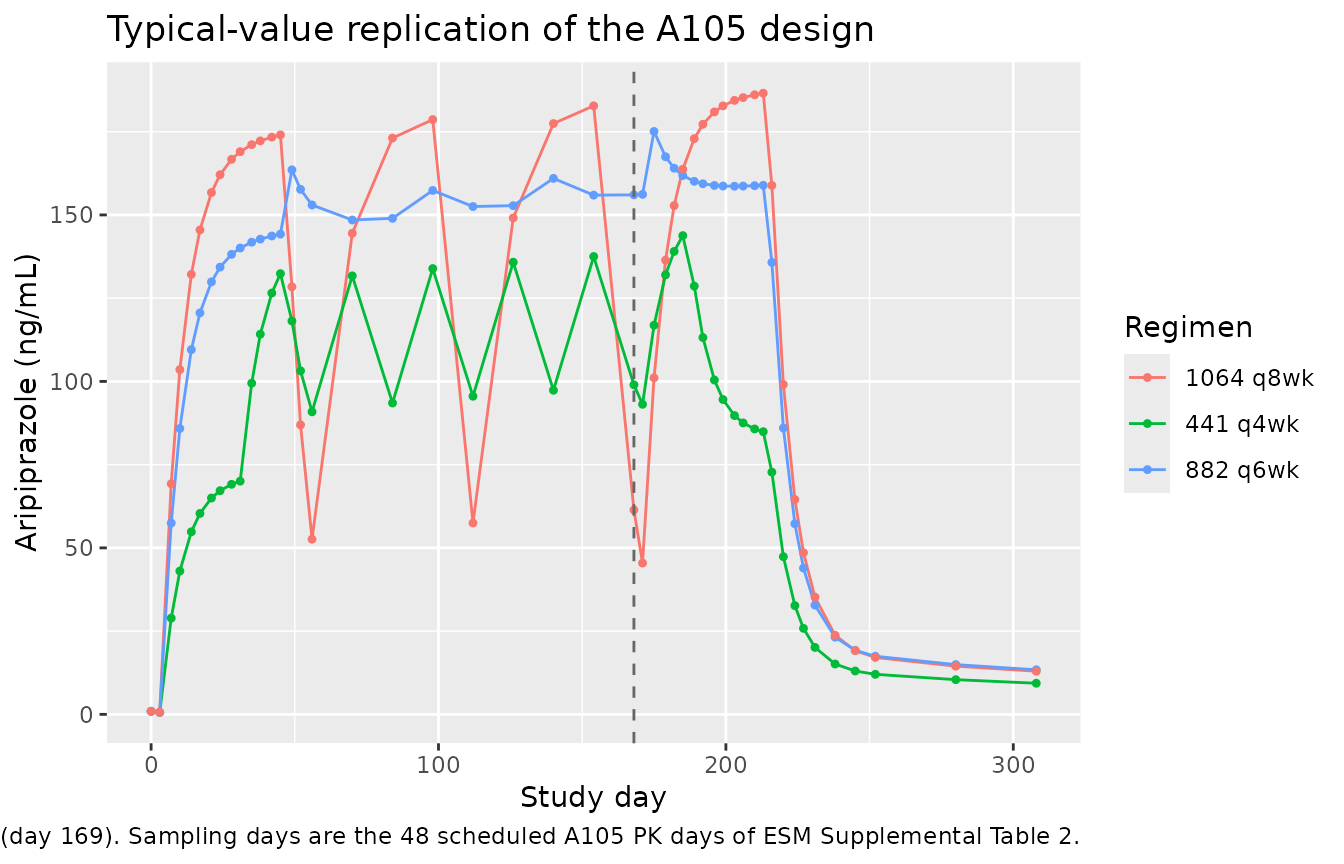
PKNCA over the interval following the last dose
The NCA frame carries time in days so the output is directly comparable with Table 2, which reports AUC in day*ng/mL and half-life in days; the model’s native time unit is hours.
nca_conc <- sim_tv |>
  dplyr::filter(!is.na(Cc)) |>
  dplyr::mutate(time_d = time / 24) |>
  dplyr::select(id, time_d, Cc, regimen)

nca_dose <- ev_tv |>
  dplyr::filter(evid == 1) |>
  dplyr::mutate(time_d = time / 24) |>
  dplyr::select(id, time_d, amt, regimen)

# Two windows per arm: the dosing interval after the last injection (Cmax,
# Tmax, Cavg, AUCtau) and the full 140-day follow-up (half-life).
intervals <- do.call(rbind, lapply(arms, function(a) {
  data.frame(
    regimen = a$regimen,
    start = c(last_dose_day - 1, last_dose_day - 1),
    end = c(last_dose_day - 1 + a$tau_d, last_dose_day - 1 + followup_day),
    cmax = c(TRUE, FALSE), tmax = c(TRUE, FALSE), cav = c(TRUE, FALSE),
    auclast = c(TRUE, FALSE), half.life = c(FALSE, TRUE)
  )
}))

conc_obj <- PKNCA::PKNCAconc(nca_conc, Cc ~ time_d | regimen + id,
                             concu = "ng/mL", timeu = "day")
dose_obj <- PKNCA::PKNCAdose(nca_dose, amt ~ time_d | regimen + id,
                             doseu = "mg")
nca_res <- suppressWarnings(
  PKNCA::pk.nca(PKNCA::PKNCAdata(conc_obj, dose_obj, intervals = intervals))
)
Comparison against the published non-compartmental analysis
# Hard 2017 Table 2, arithmetic means following the last dose.
published <- tibble::tribble(
  ~regimen,     ~cmax, ~cav, ~auclast, ~half.life,
  "441 q4wk",   161,   126,  3520,     57.2,
  "882 q6wk",   172,   131,  5510,     55.1,
  "1064 q8wk",  189,   141,  7880,     53.9
)

cmp <- nlmixr2lib::ncaComparisonTable(
  simulated = nca_res,
  reference = published,
  by = "regimen",
  units = c(cmax = "ng/mL", cav = "ng/mL", auclast = "day*ng/mL",
            half.life = "day"),
  tolerance_pct = 20
)
knitr::kable(cmp, align = c("l", "l", "r", "r", "r"),
             caption = paste("Typical-value simulation vs Hard 2017 Table 2",
"(arithmetic means).", attr(cmp, "footnote")))| NCA parameter | regimen | Reference | Simulated | % diff |
|---|---|---|---|---|
| Cmax (ng/mL) | 441 q4wk | 161 | 144 | -10.7% |
| Cmax (ng/mL) | 882 q6wk | 172 | 175 | +1.8% |
| Cmax (ng/mL) | 1064 q8wk | 189 | 187 | -1.3% |
| AUClast (day*ng/mL) | 441 q4wk | 3520 | 3370 | -4.3% |
| AUClast (day*ng/mL) | 882 q6wk | 5510 | 6780 | +23.1%* |
| AUClast (day*ng/mL) | 1064 q8wk | 7880 | 8230 | +4.5% |
| t½ (day) | 441 q4wk | 57.2 | 154 | +168.5%* |
| t½ (day) | 882 q6wk | 55.1 | 146 | +165.4%* |
| t½ (day) | 1064 q8wk | 53.9 | 140 | +160.2%* |
| Cavg (ng/mL) | 441 q4wk | 126 | 120 | -4.5% |
| Cavg (ng/mL) | 882 q6wk | 131 | 162 | +23.3%* |
| Cavg (ng/mL) | 1064 q8wk | 141 | 147 | +4.3% |
Five rows are starred, and they are two findings rather than five:
the 882 mg q6wk AUC and its Cavg (the same quantity divided by tau), and
all three half-lives. Both are discussed under Deviations below
and neither is tuned away. Cmax is reproduced in every arm,
and AUC and Cavg in the other two arms.
pct <- function(param, reg) {
  v <- cmp$`% diff`[grepl(param, cmp$`NCA parameter`, fixed = TRUE) &
                      cmp$regimen == reg]
  stopifnot(length(v) == 1L)
  abs(as.numeric(sub("%$", "", sub("\\*$", "", v))))
}

# Deterministic simulation (zeroRe on a fixed sampling grid), so these bounds
# carry no cohort-draw noise; the headroom is against the published arithmetic
# means, which come from 19-28 subjects at 40-78% CV.
stopifnot(
  pct("Cmax", "441 q4wk") < 15,
  pct("Cmax", "882 q6wk") < 15,
  pct("Cmax", "1064 q8wk") < 15,
  pct("AUClast", "441 q4wk") < 12,
  pct("AUClast", "1064 q8wk") < 12,
  pct("Cavg", "441 q4wk") < 12,
  pct("Cavg", "1064 q8wk") < 12
)
Dose linearity
The model is linear, so dose-normalised exposure over the last interval must be the same in all three arms. The published table is not – which is what the 882 mg q6wk deviation actually is.
sim_auc <- as.data.frame(nca_res$result) |>
  dplyr::filter(PPTESTCD == "auclast") |>
  dplyr::select(regimen, sim_auc = PPORRES)
eqdose <- vapply(arms, function(a) a$eq, numeric(1))
names(eqdose) <- vapply(arms, function(a) a$regimen, character(1))

lin <- published |>
  dplyr::select(regimen, pub_auc = auclast) |>
  dplyr::left_join(sim_auc, by = "regimen") |>
  dplyr::mutate(
    `Equivalent dose (mg)` = eqdose[regimen],
    `Published AUCtau / dose` = pub_auc / `Equivalent dose (mg)`,
    `Simulated AUCtau / dose` = sim_auc / `Equivalent dose (mg)`
  ) |>
  dplyr::select(regimen, `Equivalent dose (mg)`,
                `Published AUCtau / dose`, `Simulated AUCtau / dose`)
knitr::kable(lin, digits = 2,
caption = "Dose-normalised AUC over the interval after the last dose (day*ng/mL per mg aripiprazole equivalent).")| regimen | Equivalent dose (mg) | Published AUCtau / dose | Simulated AUCtau / dose |
|---|---|---|---|
| 441 q4wk | 300 | 11.73 | 11.23 |
| 882 q6wk | 600 | 9.18 | 11.31 |
| 1064 q8wk | 724 | 10.88 | 11.37 |
spread <- function(x) (max(x) - min(x)) / mean(x)
tibble::tibble(
  Source = c("Published (Table 2)", "Simulated (typical value)"),
  `Relative spread across arms` = c(spread(lin$`Published AUCtau / dose`),
                                    spread(lin$`Simulated AUCtau / dose`))
) |>
knitr::kable(digits = 4)| Source | Relative spread across arms |
|---|---|
| Published (Table 2) | 0.2406 |
| Simulated (typical value) | 0.0122 |
# The simulated arms must agree with each other to within a couple of percent --
# that is a property of a linear model, not of the cohort.
sim_spread_pct <- 100 * spread(lin$`Simulated AUCtau / dose`)
stopifnot(sim_spread_pct < 3)
Virtual cohort
# set.seed() seeds R's RNG (used for the weight draw). It does NOT seed
# rxode2's simulation RNG, whose streams are partitioned per solver thread, so
# the cohort differs between a 2-core CI runner and a 16-thread workstation.
# Every assertion below is written to hold for any cohort the model can draw.
set.seed(20260916)
n_per_arm <- 200

ev_cohort <- dplyr::bind_rows(lapply(seq_along(arms), function(i) {
  ids <- (i - 1L) * 1000L + seq_len(n_per_arm)
  # Table 1: mean +/- SD weight 89.8 +/- 16.9 kg; clipped to the earlier
  # PopPK data set's observed 43-144 kg range.
  wt <- pmin(pmax(stats::rnorm(n_per_arm, 89.8, 16.9), 43), 144)
  make_arm(arms[[i]], ids = ids, wt = wt)
}))
stopifnot(!anyDuplicated(unique(ev_cohort[, c("id", "time", "evid")])))

sim_cohort <- suppressWarnings(
  rxode2::rxSolve(ui, ev_cohort, keep = c("regimen", "WT"), addDosing = FALSE)
) |>
  as.data.frame() |>
  dplyr::filter(!is.na(Cc))

# A handful of subjects with an extreme eta draw decay into solver noise in the
# far tail and return values around -5e-10 ng/mL. That is round-off, not a
# model defect, so the assertion is on the MAGNITUDE of any negative value --
# eight orders of magnitude below the cohort median, so a genuinely negative
# prediction still goes red -- and the values are then clamped so the
# percentile bands and any log axis stay well defined.
worst_negative <- min(c(0, sim_cohort$Cc))
stopifnot(worst_negative > -1e-6)
sim_cohort$Cc <- pmax(sim_cohort$Cc, 0)
sim_cohort |>
  dplyr::group_by(regimen, time) |>
  dplyr::summarise(Q05 = quantile(Cc, 0.05), Q50 = median(Cc),
                   Q95 = quantile(Cc, 0.95), .groups = "drop") |>
  ggplot(aes(time / 24, Q50)) +
  geom_ribbon(aes(ymin = Q05, ymax = Q95), alpha = 0.22) +
  geom_line() +
  geom_line(data = sim_tv, aes(time / 24, Cc), colour = "firebrick",
            linetype = 2, inherit.aes = FALSE) +
  facet_wrap(~regimen) +
  labs(x = "Study day", y = "Aripiprazole (ng/mL)",
       title = "Simulated A105 cohort, 200 subjects per arm",
       caption = paste("Replicates the shape of Figure 1 of Hard 2017 (mean and",
                       "SD by regimen). Band = 5th-95th percentile, solid =",
                       "median, dashed red = typical-value profile. Spread is",
                       "wider than the published data because the paper's",
                       "8 x 8 OMEGA block off-diagonals are unpublished."))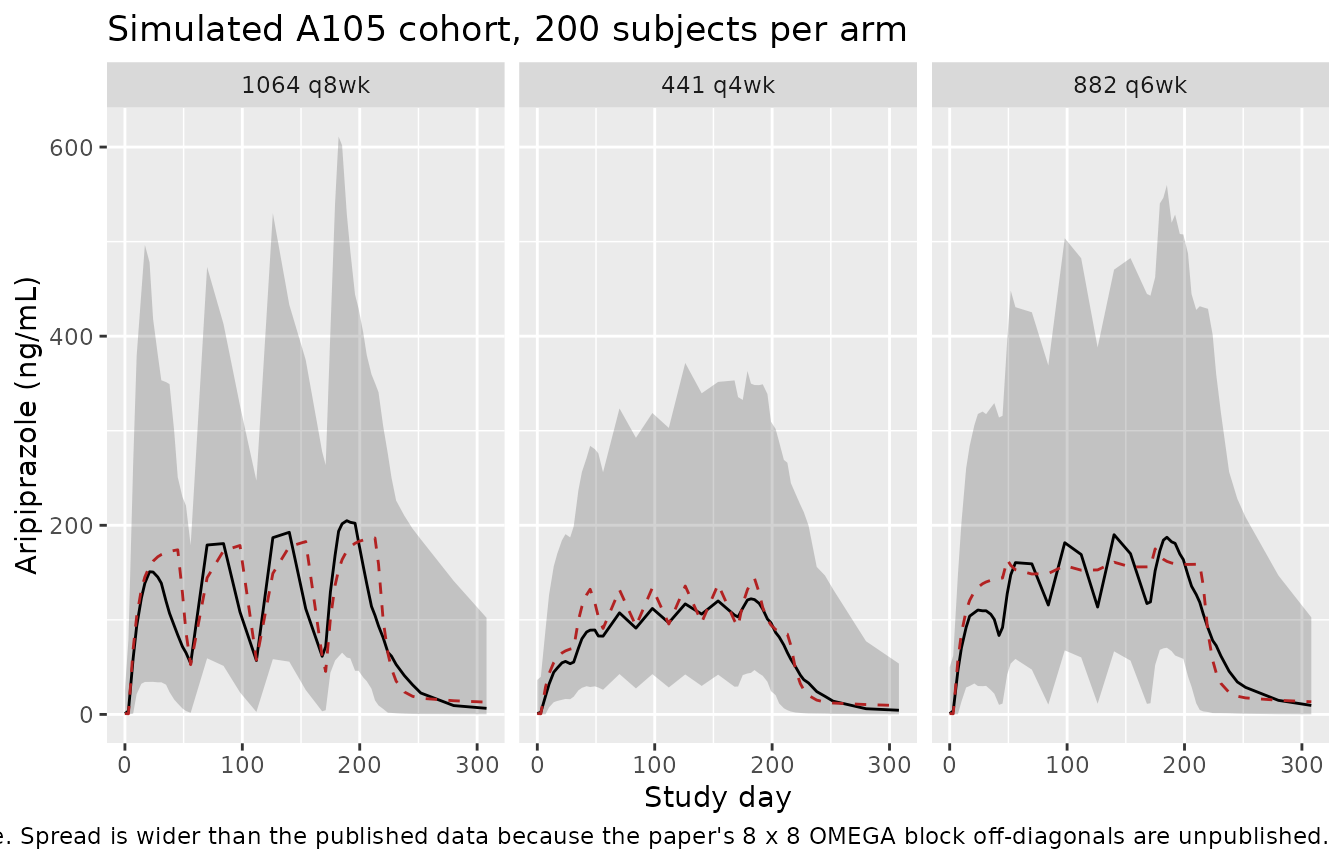
The cohort median profile should sit on the typical-value profile without a systematic offset. It does not sit on it point by point: with nine uncorrelated log-normal etas, three of which have CVs above 140%, the median subject at week 4 is not the median subject at week 40, and the resulting shape-and-timing scatter is tens of percent at any single sampling day. The check below is therefore on the median signed deviation per arm – a statistic that is near zero when the cohort is centred correctly and that moves by a factor when something structural is wrong (the classic failure being duplicate subject IDs across arms, which silently sums doses).
med <- sim_cohort |>
  dplyr::group_by(regimen, time) |>
  dplyr::summarise(Q50 = median(Cc), .groups = "drop") |>
  dplyr::inner_join(dplyr::select(sim_tv, regimen, time, Cc), by = c("regimen", "time")) |>
  dplyr::filter(time > 30 * 24) |> # after the first input has established itself
  dplyr::mutate(pct = 100 * (Q50 - Cc) / Cc)

bias <- med |>
  dplyr::group_by(regimen) |>
  dplyr::summarise(
    `Median signed % diff` = median(pct),
    `10th pct` = quantile(pct, 0.1),
    `90th pct` = quantile(pct, 0.9),
    .groups = "drop"
  )
knitr::kable(bias, digits = 2,
caption = "Cohort median profile vs the typical-value profile, across sampling days after day 30. The centre is unbiased; the per-day scatter is the shape-and-timing spread the large uncorrelated etas produce.")| regimen | Median signed % diff | 10th pct | 90th pct |
|---|---|---|---|
| 1064 q8wk | 0.09 | -43.94 | 35.94 |
| 441 q4wk | -8.74 | -30.18 | 30.31 |
| 882 q6wk | 3.15 | -26.37 | 64.29 |
# Centre only -- never the per-day extremes, which are one draw on one thread
# count. Realised -8.7 / +3.1 / +0.1 percent across the three arms here; 25
# leaves room for another draw while still going red on an id-collision bug
# (those inflate an arm by 100-300%) or a mis-scaled dose.
stopifnot(all(abs(bias$`Median signed % diff`) < 25))
Steady-state exposure across the approved regimens
Supplemental Table 4 reports simulated median steady-state Cmin /
Cmax / Cavg after 48 weeks of dosing for the four approved regimens plus
the proposed 1064 mg q8wk regimen. At true steady state a linear model’s
Cavg is fixed by mass balance at FIM * Dose / (CL/F * tau),
so the typical-value prediction can be written in closed form and
compared with the paper’s simulated medians.
ss <- tibble::tribble(
  ~regimen,       ~eq,  ~tau_d, ~pub_cavg,
  "441 mg q4wk",   300, 28,     119,
  "662 mg q4wk",   450, 28,     183,
  "882 mg q4wk",   600, 28,     249,
  "882 mg q6wk",   600, 42,     165,
  "1064 mg q8wk",  724, 56,     154
) |>
  dplyr::mutate(
    `Closed-form Cavg,ss (ng/mL)` = 1000 * fim * eq / (cl_typ * tau_d * 24),
    `% vs published median` = 100 * (`Closed-form Cavg,ss (ng/mL)` - pub_cavg) / pub_cavg
  ) |>
  dplyr::rename("Regimen" = regimen, "Aripiprazole equivalent (mg)" = eq,
                "tau (days)" = tau_d, "Published median Cavg,ss (ng/mL)" = pub_cavg)
knitr::kable(ss, digits = 1,
caption = "Closed-form steady-state Cavg from the encoded CL/F and FIM vs the simulated medians of ESM Supplemental Table 4.")| Regimen | Aripiprazole equivalent (mg) | tau (days) | Published median Cavg,ss (ng/mL) | Closed-form Cavg,ss (ng/mL) | % vs published median |
|---|---|---|---|---|---|
| 441 mg q4wk | 300 | 28 | 119 | 134.3 | 12.9 |
| 662 mg q4wk | 450 | 28 | 183 | 201.5 | 10.1 |
| 882 mg q4wk | 600 | 28 | 249 | 268.6 | 7.9 |
| 882 mg q6wk | 600 | 42 | 165 | 179.1 | 8.5 |
| 1064 mg q8wk | 724 | 56 | 154 | 162.1 | 5.2 |
Claims the paper makes about the model
claims <- tibble::tibble(
  Claim = c(
    "Duration of absorption is 43 days (ESM Suppl. Table 7 D1 = 1043 h)",
    "Lag time is 3.2 days (ESM Suppl. Table 7 ALAG = 77.5 h)",
    "Total duration of input into the systemic circulation is 46 days",
    "CL/F is reduced by 23% in CYP2D6 poor metabolizers",
    "IM bioavailability relative to oral aripiprazole is 57%"
  ),
  Achieved = c(
    sprintf("%.1f days", d1_typ / 24),
    sprintf("%.1f days", tlag_typ / 24),
    sprintf("%.1f days", (d1_typ + tlag_typ) / 24),
    sprintf("%.0f%% reduction", 100 * (1 - ui$theta[["e_cyp2d6_pm_cl"]])),
    sprintf("%.0f%%", 100 * fim)
  ),
  Pass = c(
    abs(d1_typ / 24 - 43) < 1,
    abs(tlag_typ / 24 - 3.2) < 0.2,
    abs((d1_typ + tlag_typ) / 24 - 46) < 1,
    abs(100 * (1 - ui$theta[["e_cyp2d6_pm_cl"]]) - 23) < 1,
    abs(100 * fim - 57) < 1
  )
)
knitr::kable(claims)| Claim | Achieved | Pass |
|---|---|---|
| Duration of absorption is 43 days (ESM Suppl. Table 7 D1 = 1043 h) | 43.5 days | TRUE |
| Lag time is 3.2 days (ESM Suppl. Table 7 ALAG = 77.5 h) | 3.2 days | TRUE |
| Total duration of input into the systemic circulation is 46 days | 46.7 days | TRUE |
| CL/F is reduced by 23% in CYP2D6 poor metabolizers | 23% reduction | TRUE |
| IM bioavailability relative to oral aripiprazole is 57% | 57% | TRUE |
stopifnot(is.logical(claims$Pass), !anyNA(claims$Pass), all(claims$Pass))Deviations
Three comparisons deserve comment. Two of them fall outside the 20% tolerance of the table above; the third sits inside it but is systematic enough to be worth stating. All three are recorded rather than tuned away.
1. The 882 mg q6wk arm’s observed AUC is ~19% below what a linear model predicts, and is internally inconsistent with the other two arms of the same study. Dose-normalised AUC over the last interval in Table 2 is 11.7, 9.2 and 10.9 day*ng/mL per mg aripiprazole equivalent for the 441 q4wk, 882 q6wk and 1064 q8wk arms. A linear model cannot produce that spread, and the 2MPopPK model is linear; the simulated values agree with each other to within 1.2%. The published q6wk arm has n = 19-23 with 47% CV, so its standard error is about 10% and the gap is roughly two standard errors. The model reproduces Cmax in that arm to +1.8%, so the discrepancy sits in the AUC of the observed cohort rather than in the encoded parameters.
2. The half-life implied by the model is 140-154 days against a published 54-57 days. The paper’s non-compartmental half-lives were fitted over the 140-day follow-up window, of which the first 46 days still carry input from the last injection, and their between-subject CVs are 58-78%. The model’s own terminal eigenvalue (computed above) is a 178-day beta phase, driven by Vp/F = 2122 L and Q/F = 0.423 L/h. Those two parameters were not estimated by the 2MPopPK model: ESM Supplemental Table 7 footnote a fixes them at the earlier PopPK model’s values, where the deep compartment was fitted jointly with dehydro-aripiprazole. The 2MPopPK model dropped dehydro-aripiprazole but kept the disposition parameters, so its terminal phase is inherited rather than re-identified from these data. Use the model for the exposure metrics it was built for (Cmax, Cavg, AUC over a dosing interval), not for terminal half-life.
3. The closed-form steady-state Cavg runs 5-13% above the simulated medians of Supplemental Table 4. The offset is largest for the q4wk regimens and smallest for q8wk. Mass balance fixes Cavg at steady state, so the paper’s simulated medians must reflect something other than a fully-converged steady state – plausibly the 48-week simulation horizon against the model’s very slow terminal phase, or the seven-depot ceiling of the NONMEM implementation (a 48-week q4wk course needs 13 injections but the published model carries only seven IM depots, whereas the q8wk course needs only seven).
Assumptions and deviations
Weight centering (70 kg) comes from the earlier paper, not this one. The 2MPopPK paper states only that the weight effect on Vc/F was “retained” from the earlier PopPK model and never prints the centering value. Hard 2017 J Clin Psychopharmacol Supplementary Data Content states it explicitly (“centered for a weight of 70 kg”) and prints
VC/F = 268*(WT/70)^1.0. That paper is the direct predecessor, is cited as reference 2 of the ESM, and supplies the values of Vp/F, Q/F and ARI(0) that the 2MPopPK model fixed, so it is the authoritative source for the centering constant too.Ka and FIM are encoded as estimated, not fixed, against two prose statements to the contrary. ESM Sect. 4 and the main paper’s Discussion both say the oral-related parameters “were fixed to the estimates obtained from the earlier PopPK model”. Supplemental Table 7 disagrees:
KaandFIMcarry %RSE and 95% CIs and are not marked with the**fixed flag that VP/F, Q/F, ARI(0), FPO and the WT exponent all carry. The earlier model’s values settle it – its Ka is 0.574 1/h and its FIM (Formulation 2) is 0.581, whereas the 2MPopPK values are 0.803 and 0.571. Values that differ from the ones they were supposedly fixed to were re-estimated. The prose most likely describes the base-model step, before those parameters were freed.The off-diagonals of the 8 x 8 OMEGA block are unpublished. ESM Sect. 4 states that IIV on eight of the structural parameters was estimated “in an OMEGA block”, but Supplemental Table 7 prints only the diagonal variances. The model therefore encodes diagonal IIV only. Typical-value predictions are unaffected; simulated between-subject spread is wider than the paper’s, most visibly for the long dosing intervals where the large, uncorrelated Q/F (CV 145%) and Vp/F (CV 435%) variabilities are free to move independently of clearance. Do not read the cohort percentile bands above as a reproduction of the paper’s VPCs.
The seven IM depots are encoded as one lagged zero-order input to
central. They are mathematically equivalent by superposition (verified by the overlapping-input mass-balance check above), and the encoded form has no seven-injection ceiling. The trade-off is thatf(central)now carries FIM, so a hypothetical intravenous dose written tocentralwould also be scaled by 0.571; the published data set contains no intravenous route.ARI(0)is encoded as an initial condition oncentral, not as an additive offset on the prediction. The(0)notation is NONMEM’s initial-amount syntax and the earlier paper’s abbreviation list reads “ARI(0), baseline amount of ARI”; both tables report it in ng/mL, so the encoding iscentral(0) <- c0 * vc / 1000. It decays with the disposition, which is the behaviour a residual pre-study oral dose should have. Its IIV variance of 5.89 is very large (the table’s own CV is 1898%); users simulating the first weeks after a first injection should be aware that a small number of virtual subjects will start with a substantial residual concentration.FPO’s IIV was fixed to zero (ESM Sect. 4), so no eta is attached tolfdepot.Inter-occasion variability is encoded over seven occasions. The paper reports a single IOV variance on
D1and its model carried seven IM depots, so seven occasion slots are encoded with occasions 2-7 fixed to the occasion-1 estimate, the NONMEMOMEGA BLOCK(1) SAMEidiom. A data set with more than seven injections should either recycleOCCor acceptOCC = 0(no IOV) on the later records.No covariate effects beyond weight-on-Vc/F and CYP2D6-on-CL/F. The full model also carried surface area on D1, ALAG and FIM, and race and sex on CL/F; ESM Supplemental Table 3 reports all seven. None of the five additional effects reduced the objective function value and all were dropped, so they are not encoded. They are recorded in the model file’s
covariateDatanotes only where they overlap a retained covariate.The virtual cohort’s weight distribution is drawn as
N(89.8, 16.9)kg (Table 1 of the phase I study) and clipped to the 43-144 kg range the earlier PopPK data set spanned. The simulated cohorts are all CYP2D6 non-poor-metabolizers and all flaggedSTUDY_A105 = 1, matching the arm being replicated.